Slide Graph Pipeline
Click to open in: [GitHub][Colab]
Introduction
Note: This notebook is aimed at advanced users who are interested in using TIAToolbox as part of an experiment or larger project.
Note: This notebook is a simplified inference portion of a larger notebook which is available here Slide Graph Pipeline. This larger notebook contains a full pipeline (training and inference) to reproduce the results of the method referenced here.
Here we demonstrate how the inference in the method of “SlideGraph+: Whole Slide Image Level Graphs to Predict HER2Status in Breast Cancer” by Lu et al. (2021) can be done using the functionalities available in TIAToolbox. As a brief overview, this method involves generating a graph to represent a whole slide image (WSI) level and then directly using it as input to predict a slide level label. For this notebook, our task is to classify a whole slide image (WSI) as HER2 negative or positive. We will use a sample WSI from TCGA-BRCA and a model pretrained on the TCGA-BRCA dataset.
Throughout this notebook we use modules from TIAToolbox to assist with standard tasks including:
Patch extraction
Stain normalization
Cell segmentation & classification
Extraction of deep features
Graph Construction
Graph Plotting
Note: Although the original paper was evaluated for HER2. The method itself can be applicable for other mutation prediction. We provide a pretrained model for predicting ER (Estrogen receptor) status here (model weights) and here (model auxiliary). You can get the pre-generated graphs here and its node preprocessing model here. For predicting ER status, we use deep features coming from ResNet50 rather than the cellular composition.
Preparation: Imports, Helpers, & Data Split
We begin by importing some libraries, defining some helper functions and defining how we will split the dataset into train, validation, and test sets.
Import Libraries
"""Import modules required to run the Jupyter notebook."""

from __future__ import annotations

# Clear logger to use tiatoolbox.logger
import logging
import sys

if logging.getLogger().hasHandlers():
    logging.getLogger().handlers.clear()

# Python standard library imports
import json
import pathlib
import random
import shutil
import warnings
from pathlib import Path
from typing import TYPE_CHECKING

# Third party imports
import joblib
import matplotlib as mpl
import matplotlib.pyplot as plt
import numpy as np
import torch
import torch.nn.functional as F  # noqa: N812
from shapely.geometry import box as shapely_box
from shapely.strtree import STRtree
from skimage.exposure import equalize_hist
from sklearn.decomposition import PCA
from sklearn.preprocessing import StandardScaler
from torch import nn
from torch.nn import BatchNorm1d, Linear, ReLU
from torch_geometric.data import Batch, Data
from torch_geometric.nn import (
    EdgeConv,
    GINConv,
    global_add_pool,
    global_max_pool,
    global_mean_pool,
)

from tiatoolbox import logger
from tiatoolbox.data import stain_norm_target
from tiatoolbox.models import (
    DeepFeatureExtractor,
    IOSegmentorConfig,
    NucleusInstanceSegmentor,
)
from tiatoolbox.models.architecture.vanilla import CNNBackbone
from tiatoolbox.tools.graph import SlideGraphConstructor
from tiatoolbox.tools.patchextraction import PatchExtractor
from tiatoolbox.tools.stainnorm import get_normalizer
from tiatoolbox.utils.misc import download_data
from tiatoolbox.utils.visualization import plot_graph
from tiatoolbox.wsicore.wsireader import WSIReader

if "google.colab" in sys.modules:
    from google.colab import output

    output.enable_custom_widget_manager()
    logger.info("Custom widget manager enabled in Google Colab environment.")

if TYPE_CHECKING:
    from collections.abc import Callable

    from tiatoolbox.wsicore.wsimeta import Resolution, Units

warnings.filterwarnings("ignore")
mpl.rcParams["figure.dpi"] = 300  # for high resolution figure in notebook
mpl.rcParams["figure.facecolor"] = "white"  # To make sure text is visible in dark mode
Helper Functions
Here we define some helper functions that will be used throughout the notebook:
def load_json(path: str) -> dict | list | int | float | str:
    """Load JSON from a file path."""
    with path.open() as fptr:
        return json.load(fptr)


def rmdir(dir_path: str) -> None:
    """Remove a directory."""
    if dir_path.is_dir():
        shutil.rmtree(dir_path)


def rm_n_mkdir(dir_path: str) -> None:
    """Remove then re-create a directory."""
    if dir_path.is_dir():
        shutil.rmtree(dir_path)
    dir_path.mkdir(parents=True)


def mkdir(dir_path: str) -> None:
    """Create a directory if it does not exist."""
    if not dir_path.is_dir():
        dir_path.mkdir(parents=True)
Fixing Randomness
We fix the random generator to 1) make debugging easier, and 2) enable us to test whether our pipeline has the same properties as the pipeline that we are trying to reproduce. (For this comparison to work, the original pipeline needs to be constructed using the same random seed.)
SEED = 5
random.seed(SEED)
rng = np.random.default_rng(SEED)
torch.manual_seed(SEED)
torch.cuda.manual_seed(SEED)
Loading Data
Here we define the sample data used for this notebook.
By default, the code checks for the existence of the folder DOWNLOAD_DIR.
If this folder does not exist, the code will download the data that we prepared beforehand.
If you want to store the intermediate results at a different location,
you need to edit WORKSPACE_DIR accordingly.
Other than that, the pre-trained models can be found using the following path variables, giving locations of models described in the larger notebook mentioned previously:
SCALER_PATH: The model to standardize the features of each node within the WSI graph.MODEL_WEIGHTS_PATH: The weights of the graph neural network.MODEL_AUX_PATH: The model to calibrate the model predictions into proper probabilities.
WORKSPACE_DIR = Path("./workspace")
DOWNLOAD_DIR = WORKSPACE_DIR / "download"

WSI_PATH = DOWNLOAD_DIR / "sample.svs"
MSK_PATH = DOWNLOAD_DIR / "sample_mask.png"
PRE_GENERATED_GRAPH_PATH = DOWNLOAD_DIR / "graph.json"
SCALER_PATH = DOWNLOAD_DIR / "node_scaler.dat"
MODEL_WEIGHTS_PATH = DOWNLOAD_DIR / "model.weigths.pth"
MODEL_AUX_PATH = DOWNLOAD_DIR / "model.aux.dat"
# ! Uncomment this to always download data
rmdir(DOWNLOAD_DIR)

# Downloading sample image tile
if not DOWNLOAD_DIR.exists():
    DOWNLOAD_DIR.mkdir(parents=True)
    URL_HOME = (
        "https://tiatoolbox.dcs.warwick.ac.uk/models/slide_graph/cell-composition"
    )
    SLIDE_CODE = "TCGA-C8-A278-01Z-00-DX1.188B3FE0-7B20-401A-A6B7-8F1798018162"
    download_data(f"{URL_HOME}/{SLIDE_CODE}.svs", WSI_PATH)
    download_data(f"{URL_HOME}/{SLIDE_CODE}.mask.png", MSK_PATH)
    download_data(f"{URL_HOME}/{SLIDE_CODE}.json", PRE_GENERATED_GRAPH_PATH)
    download_data(f"{URL_HOME}/node_scaler.dat", SCALER_PATH)
    download_data(f"{URL_HOME}/model.aux.logistic.dat", MODEL_AUX_PATH)
    download_data(f"{URL_HOME}/model.weights.pth", MODEL_WEIGHTS_PATH)
Generating a Graph from a WSI
Note: If you do not want to construct the graphs and only want to try out the graph neural network portion, we provide pre-generated graphs based on cell-composition features extracted from HoVer-Net at this link. After downloading and extracting them, please follow the instructions below for how to proceed after the graphs have been constructed.
We represent each WSI as a graph. Each node in the graph corresponds to one local region (such as image patch) within the WSI and is then represented by a set of features. Here, we describe two possible alternative feature representations, that have been found to be useful. Users might want to use other feature representations different from both of these:
Deep Neural Network features: obtained from the global average pooling layer after we apply ResNet50 on the image patch.
Cellular composition: where we count the number of nuclei of each type within the patch. The pre-trained model (HoVer-Net trained on Pannuke), available from TIAToolbox, recognizes the following nucleus types: neoplastic, non-neoplastic epithelial, inflammatory, connective tissue and necrotic.
With these node-level representations (or features), we then perform clustering so that nodes that are close to each other both in feature space and in the 2D space (i.e the WSI canvas) are assigned to the same cluster. These clusters are then linked to other clusters within a certain distance, thus giving a WSI graph.
Note: Features of patches and their positions within each WSI will be stored separately in files named
*.features.npyand*.position.npy*. Thepositionof a feature is, by definition, the patch bounding box(start_x, start_y, end_x, end_y)at the highest resolution. Subsequent function definitions will be based upon this convention.
Deep Feature Extraction
We now show how to use the toolbox to extract features. For better organization, we package
the task into a small function called extract_deep_features.
In this function, we construct the config object which defines the shape and magnification of the
patch we want to extract. Although the patches are allowed to have arbitrary size and differing
resolutions, here we use a patch of size 512x512 with 0.25 microns-per-pixel (mpp=0.25).
We use ResNet50 trained on ImageNet as a feature extractor. For more
detail on how to further customize this, you can refer to this notebook.
We explain how to construct a customized preprocessing function that we would like
the engine to perform on each input patch. (By an engine, we mean one of the top
level classes defined in one of the functions in the module tiatoolbox.models.engine.
Each instance of such a class has multiple properties and abilities, possibly
incorporating several functions.) For this notebook, we perform stain-normalization
on each image patch. Later we show how this function can be defined.
By default, the names of output files from the toolbox are
changed to sequentially ordered names (000.*.npy, 001.*.npy, etc.) to avoid
inadvertent overwriting. A mapping from output path name to input path name
is returned by the engine, making the name change easy to manage.
In this demo, we use a toolbox model with only one head (output channel).
For each input, we obtain files *.position.npy and *.features.0.npy.
(The wildcards ‘*’ are, by default replaced by sequentially ordered names as just explained.)
In the case of models having multiple output heads (output channels), the output is
['*.position.npy', '*.features.0.npy', '*.features.1.npy', etc.].
The positions are always defined as the patch bounding box (start_x, start_y, end_x, end_y)
at the highest resolution within the list of input resolutions.
Refer to the semantic segmentation notebook) for details.
def extract_deep_features(
    wsi_paths: list[str],
    msk_paths: list[str],
    save_dir: str,
    preproc_func: Callable | None = None,
) -> list:
    """Helper function to extract deep features."""
    ioconfig = IOSegmentorConfig(
        input_resolutions=[
            {"units": "mpp", "resolution": 0.25},
        ],
        output_resolutions=[
            {"units": "mpp", "resolution": 0.25},
        ],
        patch_input_shape=[512, 512],
        patch_output_shape=[512, 512],
        stride_shape=[512, 512],
        save_resolution={"units": "mpp", "resolution": 8.0},
    )
    model = CNNBackbone("resnet50")  # TimmBackbone(backbone="UNI", pretrained=True)
    extractor = DeepFeatureExtractor(batch_size=32, model=model, num_loader_workers=4)
    # Injecting customized preprocessing functions,
    # check the document or sample code below for API.
    extractor.model.preproc_func = preproc_func

    rmdir(save_dir)
    output_map_list = extractor.predict(
        wsi_paths,
        msk_paths,
        mode="wsi",
        ioconfig=ioconfig,
        device=device,
        crash_on_exception=True,
        save_dir=save_dir,
    )

    # Rename output files
    for input_path, output_path in output_map_list:
        input_name = Path(input_path).stem

        output_parent_dir = pathlib.Path(output_path).parent

        src_path = pathlib.Path(f"{output_path}.position.npy")
        new_path = pathlib.Path(f"{output_parent_dir}/{input_name}.position.npy")
        src_path.rename(new_path)

        src_path = pathlib.Path(f"{output_path}.features.0.npy")
        new_path = pathlib.Path(f"{output_parent_dir}/{input_name}.features.npy")
        src_path.rename(new_path)

    return output_map_list
Cell Composition Extraction
In a similar manner, we define the code to extract cell
composition in extract_composition_features. First, we need to
detect all nuclei in the WSI and their types. This can be
easily achieved via the tiatoolbox.models.NucleusInstanceSegmentor
engine and the HoVer-Net pretrained model, both provided in the toolbox.
Once we have the nuclei, we split the WSI into patches
and count the nuclei of each type in each patch.
We encapsulate this process in the function get_composition_features.
Unlike the DeepFeatureExtractor above, the NucleusInstanceSegmentor engine
returns a single output file given a single WSI input. The corresponding output
files are named as ['*/0.dat', '*/1.dat', etc.]. Each of these .dat files is used to generate
two files named *.features.npy and *.position.npy. As in the case of DeepFeatureExtractor,
the wildcard _* is, by default, replaced by sequentially ordered names,
for easier management and to avoid inadvertent overwriting.
def get_cell_compositions(
    wsi_path: str,
    mask_path: str,
    inst_pred_path: str,
    save_dir: str,
    num_types: int = 6,
    patch_input_shape: tuple[int] = (512, 512),
    stride_shape: tuple[int] = (512, 512),
    resolution: Resolution = 0.25,
    units: Units = "mpp",
) -> None:
    """Estimates cellular composition."""
    reader = WSIReader.open(wsi_path)
    inst_pred = joblib.load(inst_pred_path)
    # Convert to {key: int, value: dict}
    inst_pred = {i: v for i, (_, v) in enumerate(inst_pred.items())}

    inst_boxes = [v["box"] for v in inst_pred.values()]
    inst_boxes = np.array(inst_boxes)

    geometries = [shapely_box(*bounds) for bounds in inst_boxes]
    spatial_indexer = STRtree(geometries)

    # * Generate patch coordinates (in xy format)
    wsi_shape = reader.slide_dimensions(resolution=resolution, units=units)

    (patch_inputs, _) = PatchExtractor.get_coordinates(
        image_shape=wsi_shape,
        patch_input_shape=patch_input_shape,
        patch_output_shape=patch_input_shape,
        stride_shape=stride_shape,
    )

    # Filter out coords which dont lie in mask
    selected_coord_indices = PatchExtractor.filter_coordinates(
        WSIReader.open(mask_path),
        patch_inputs,
        wsi_shape=wsi_shape,
        min_mask_ratio=0.5,
    )
    patch_inputs = patch_inputs[selected_coord_indices]

    bounds_compositions = []
    for bounds in patch_inputs:
        bounds_ = shapely_box(*bounds)
        indices = [
            geo
            for geo in spatial_indexer.query(bounds_)
            if bounds_.contains(geometries[geo])
        ]
        insts = [inst_pred[v]["type"] for v in indices]
        uids, freqs = np.unique(insts, return_counts=True)
        # A bound may not contain all types, hence, to sync
        # the array and placement across all types, we create
        # a holder then fill the count within.
        holder = np.zeros(num_types, dtype=np.int16)
        holder[uids.astype(int)] = freqs
        bounds_compositions.append(holder)
    bounds_compositions = np.array(bounds_compositions)

    base_name = pathlib.Path(wsi_path).stem
    # Output in the same saving protocol for construct graph
    np.save(f"{save_dir}/{base_name}.position.npy", patch_inputs)
    np.save(f"{save_dir}/{base_name}.features.npy", bounds_compositions)


def extract_composition_features(
    wsi_paths: list[str],
    msk_paths: list[str],
    save_dir: str,
    preproc_func: Callable,
) -> list:
    """Extract cellular composition features."""
    inst_segmentor = NucleusInstanceSegmentor(
        pretrained_model="hovernet_fast-pannuke",
        batch_size=16,
        num_postproc_workers=4,
        num_loader_workers=4,
    )
    # bigger tile shape for postprocessing performance
    inst_segmentor.ioconfig.tile_shape = (4000, 4000)
    # Injecting customized preprocessing functions,
    # check the document or sample codes below for API
    inst_segmentor.model.preproc_func = preproc_func

    rmdir(save_dir)
    output_map_list = inst_segmentor.predict(
        wsi_paths,
        msk_paths,
        mode="wsi",
        device=device,
        crash_on_exception=True,
        save_dir=save_dir,
    )
    # Rename output files of toolbox
    output_paths = []
    for input_path, output_path in output_map_list:
        input_name = pathlib.Path(input_path).stem

        output_parent_dir = pathlib.Path(output_path).parent

        src_path = pathlib.Path(f"{output_path}.dat")
        new_path = pathlib.Path(f"{output_parent_dir}/{input_name}.dat")
        src_path.rename(new_path)
        output_paths.append(new_path)

    # TODO(TBC): Parallelize this if possible  # noqa: TD003, FIX002
    for idx, path in enumerate(output_paths):
        get_cell_compositions(wsi_paths[idx], msk_paths[idx], path, save_dir)
    return output_paths
Apply Stain Normalization Across Image Patches
Extracting either deep features or cell compositions above requires inference on each patch within the WSI. In histopathology, we often want to normalize the image patch staining to reduce variation as much as possible.
Here we define the normalizer and a function to perform normalisation later
in parallel processing manner. The target image and the normalizer are
provided at tiatoolbox.tools.stainnorm and tiatoolbox.data.
We do not perform stain normalisation at this point in the program. Instead, we
stain-normalize in tandem with other methods in the toolbox during pre-processing.
In our case, this will be done by the engine object defined above.
target_image = stain_norm_target()
stain_normaliser = get_normalizer("reinhard")
stain_normaliser.fit(target_image)


def stain_norm_func(img: np.ndarray) -> np.ndarray:
    """Helper function to perform stain normalization."""
    return stain_normaliser.transform(img)
Constructing the Graphs
Above, we have already defined functions that can perform WSI feature extraction.
Now we perform the extraction itself and save the results in WSI_FEATURE_DIR for
later graph construction. The particular patch features to be extracted are controlled
by the FEATURE_MODE variable. At present we support two alternatives:
"cnn": for the deep neural network features. We use ResNet50 pretrained on ImageNet as feature extractor. Therefore, there are 2048 features representing each image patch. The patches as well as the resulting nodes are atmpp=0.25."composition": for the cell composition features. The features here are the counts of each nuclei type within the image. We use the HoVer-Net pretrained on Pannuke data to identify 6 nuclei types: neoplastic epithelial, lymphocytes, connective tissue, necrosis, and non-neoplastic epithelial. The patches as well as the resulting nodes are atmpp=0.25.
Once the patches and their features are extracted, we construct a graph for the sample WSI
by using the function provided in tiatoolbox.tools.graph. Here, each node in the WSI graph
corresponds to a patch (or local region) which we obtain from the extraction process.
You can change where the graph is saved by editing GRAPH_PATH.
Lastly, feature extraction process may take a long time depending on the type
of patch feature to be extracted. In particular, for a WSI of size 60k x 60k,
"cnn" takes around three minutes, while "composition" may take over an hour.
By default, USE_PRE_GENERATED = True and we use the graph
we previously downloaded for subsequent steps. However, you can try out
the entire process by setting USE_PRE_GENERATED = False.
Note: In this notebook, each node of the graph represents a patch. However, if you prefer, you can provide your own version of nodes and their features. You will need to modify the lines
positions = np.load(f"{WSI_FEATURE_DIR}/{wsi_name}.position.npy")
features = np.load(f"{WSI_FEATURE_DIR}/{wsi_name}.features.npy")
within
construct_graphto fit with your objectives.
Note: Each node within the pre-generated graphs has 4 features where each corresponds to the number of a specific nuclei type within the image patch. For this graph, they are neoplastic epithelial, non-neoplastic epithelial, inflammatory, and connective tissue respectively. Lastly, these image patches as well as the resulting nodes were obtained at
mpp=0.50.
# ! for trying out the function

# ! for trying out the function

# ! for using pre-generated graph
NUM_NODE_FEATURES = 4
FEATURE_MODE = "composition"
USE_PRE_GENERATED = True

WSI_FEATURE_DIR = WORKSPACE_DIR / "features/"
GRAPH_PATH = WORKSPACE_DIR / "graph.json"
def construct_graph(wsi_name: str, save_path: str | Path) -> None:
    """Construct graph for one WSI and save to file."""
    positions = np.load(f"{WSI_FEATURE_DIR}/{wsi_name}.position.npy")
    features = np.load(f"{WSI_FEATURE_DIR}/{wsi_name}.features.npy")
    graph_dict = SlideGraphConstructor.build(
        positions[:, :2],
        features,
        feature_range_thresh=None,
    )

    # Write a graph to a JSON file
    with save_path.open("w") as handle:
        graph_dict = {k: v.tolist() for k, v in graph_dict.items()}
        json.dump(graph_dict, handle)


# Generate node features
if not USE_PRE_GENERATED:
    if FEATURE_MODE == "composition":
        output_list = extract_composition_features(
            [WSI_PATH],
            [MSK_PATH],
            WSI_FEATURE_DIR,
            stain_norm_func,
        )
    else:
        output_list = extract_deep_features(
            [WSI_PATH],
            [MSK_PATH],
            WSI_FEATURE_DIR,
            stain_norm_func,
        )

    wsi_name = pathlib.Path(WSI_PATH).stem
    GRAPH_PATH = f"{WORKSPACE_DIR}/{wsi_name}.json"

    # Build up the graph
    construct_graph(wsi_name, GRAPH_PATH)

GRAPH_PATH = GRAPH_PATH if not USE_PRE_GENERATED else PRE_GENERATED_GRAPH_PATH
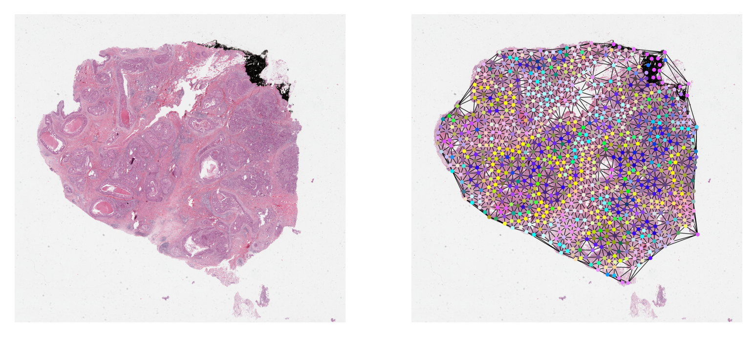
Visualize a Graph
It is always a good practice to validate data and any results visually.
Here, we plot the sample graph upon its WSI thumbnail. When plotting,
the nodes within the graph will often be at different resolution
from the resolution at which we want to visualize them. We scale their coordinates
to the target resolution before plotting. We provide NODE_RESOLUTION and PLOT_RESOLUTION variables
respectively as the resolution of the node and the resolution at which to plot the graph.
NODE_SIZE = 24
if USE_PRE_GENERATED:
    NODE_RESOLUTION = {"resolution": 0.5, "units": "mpp"}
else:
    NODE_RESOLUTION = {"resolution": 0.25, "units": "mpp"}
PLOT_RESOLUTION = {"resolution": 4.00, "units": "mpp"}
graph_dict = load_json(GRAPH_PATH)
graph_dict = {k: np.array(v) for k, v in graph_dict.items()}
graph = Data(**graph_dict)

# deriving node colors via projecting n-d features down to 3-d
graph.x = StandardScaler().fit_transform(graph.x)
# .c for node colors
node_colors = PCA(n_components=3).fit_transform(graph.x)[:, [1, 0, 2]]
for channel in range(node_colors.shape[-1]):
    node_colors[:, channel] = 1 - equalize_hist(node_colors[:, channel]) ** 2
node_colors = (node_colors * 255).astype(np.uint8)

reader = WSIReader.open(WSI_PATH)
thumb = reader.slide_thumbnail(4.0, "mpp")

node_resolution = reader.slide_dimensions(**NODE_RESOLUTION)
plot_resolution = reader.slide_dimensions(**PLOT_RESOLUTION)
fx = np.array(node_resolution) / np.array(plot_resolution)

if USE_PRE_GENERATED:
    node_coordinates = np.array(graph.coords) / fx
else:
    node_coordinates = np.array(graph.coordinates) / fx
edges = graph.edge_index.T

thumb = reader.slide_thumbnail(**PLOT_RESOLUTION)
thumb_overlaid = plot_graph(
    thumb.copy(),
    node_coordinates,
    edges,
    node_colors=node_colors,
    node_size=NODE_SIZE,
)

plt.subplot(1, 2, 1)
plt.imshow(thumb)
plt.axis("off")
plt.subplot(1, 2, 2)
plt.imshow(thumb_overlaid)
plt.axis("off")
plt.show()
Graph Neural Network
class SlideGraphArch(nn.Module):
    """Define SlideGraph architecture."""

    def __init__(
        self: nn.Module,
        dim_features: int,
        dim_target: int,
        layers: tuple[int, int] | None = None,
        pooling: str = "max",
        dropout: int = 0.0,
        conv: str = "GINConv",
        *,
        gembed: bool = False,
        **kwargs: dict,
    ) -> None:
        """Initialize SlideGraphArch."""
        super().__init__()
        if layers is None:
            layers = [6, 6]
        self.dropout = dropout
        self.embeddings_dim = layers
        self.num_layers = len(self.embeddings_dim)
        self.nns = []
        self.convs = []
        self.linears = []
        self.pooling = {
            "max": global_max_pool,
            "mean": global_mean_pool,
            "add": global_add_pool,
        }[pooling]
        # If True then learn a graph embedding for final classification
        # (classify pooled node features), otherwise pool node decision scores.
        self.gembed = gembed

        conv_dict = {"GINConv": [GINConv, 1], "EdgeConv": [EdgeConv, 2]}
        if conv not in conv_dict:
            msg = f'Not support `conv="{conv}".'
            raise ValueError(msg)

        def create_linear(in_dims: int, out_dims: int) -> Linear:
            return nn.Sequential(
                Linear(in_dims, out_dims),
                BatchNorm1d(out_dims),
                ReLU(),
            )

        input_emb_dim = dim_features
        out_emb_dim = self.embeddings_dim[0]
        self.first_h = create_linear(input_emb_dim, out_emb_dim)
        self.linears.append(Linear(out_emb_dim, dim_target))

        input_emb_dim = out_emb_dim
        for out_emb_dim in self.embeddings_dim[1:]:
            conv_class, alpha = conv_dict[conv]
            subnet = create_linear(alpha * input_emb_dim, out_emb_dim)
            # ! this variable should be removed after training integrity checking
            self.nns.append(subnet)  # <--| as it already within ConvClass
            self.convs.append(conv_class(self.nns[-1], **kwargs))
            self.linears.append(Linear(out_emb_dim, dim_target))
            input_emb_dim = out_emb_dim

        self.nns = torch.nn.ModuleList(self.nns)
        self.convs = torch.nn.ModuleList(self.convs)
        # Has got one more for initial input, what does this mean
        self.linears = torch.nn.ModuleList(self.linears)

        # Auxilary holder for external model, these are saved separately from torch.save
        # as they can be sklearn model etc.
        self.aux_model = {}

    def save(self: nn.Module, path: str | Path, aux_path: str | Path) -> None:
        """Save torch model."""
        state_dict = self.state_dict()
        torch.save(state_dict, path)
        joblib.dump(self.aux_model, aux_path)

    def load(self: nn.Module, path: str | Path, aux_path: str | Path) -> None:
        """Load torch model."""
        state_dict = torch.load(path)
        self.load_state_dict(state_dict)
        self.aux_model = joblib.load(aux_path)

    def forward(
        self: nn.Module,
        data: torch.Tensor,
    ) -> tuple[torch.Tensor, torch.Tensor]:
        """Torch model forward function."""
        feature, edge_index, batch = (
            data.x,
            data.edge_index.type(torch.int64),
            data.batch,
        )

        wsi_prediction = 0
        pooling = self.pooling
        node_prediction = 0

        feature = self.first_h(feature)
        for layer in range(self.num_layers):
            if layer == 0:
                node_prediction_sub = self.linears[layer](feature)
                node_prediction += node_prediction_sub
                node_pooled = pooling(node_prediction_sub, batch)
                wsi_prediction_sub = F.dropout(
                    node_pooled,
                    p=self.dropout,
                    training=self.training,
                )
                wsi_prediction += wsi_prediction_sub
            else:
                feature = self.convs[layer - 1](feature, edge_index)
                if not self.gembed:
                    node_prediction_sub = self.linears[layer](feature)
                    node_prediction += node_prediction_sub
                    node_pooled = pooling(node_prediction_sub, batch)
                    wsi_prediction_sub = F.dropout(
                        node_pooled,
                        p=self.dropout,
                        training=self.training,
                    )
                else:
                    node_pooled = pooling(feature, batch)
                    node_prediction_sub = self.linears[layer](node_pooled)
                    wsi_prediction_sub = F.dropout(
                        node_prediction_sub,
                        p=self.dropout,
                        training=self.training,
                    )
                wsi_prediction += wsi_prediction_sub
        return wsi_prediction, node_prediction

    # Run one single step
    @staticmethod
    def train_batch(
        model: nn.Module,
        batch_data: torch.Tensor,
        optimizer: torch.optim.Optimizer,
        device: str,
    ) -> list:
        """Helper function for model training."""
        wsi_graphs = batch_data["graph"].to(device)
        wsi_labels = batch_data["label"].to(device)
        model = model.to(device)

        # Data type conversion
        wsi_graphs.x = wsi_graphs.x.type(torch.float32)

        # Not an RNN so does not accumulate
        model.train()
        optimizer.zero_grad()

        wsi_output, _ = model(wsi_graphs)

        # Both are expected to be Nx1
        wsi_labels_ = wsi_labels[:, None]
        wsi_labels_ = wsi_labels_ - wsi_labels_.T
        wsi_output_ = wsi_output - wsi_output.T
        diff = wsi_output_[wsi_labels_ > 0]
        loss = torch.mean(F.relu(1.0 - diff))
        # Backprop and update
        loss.backward()
        optimizer.step()

        loss = loss.detach().cpu().numpy()
        assert not np.isnan(loss)  # noqa: S101
        wsi_labels = wsi_labels.cpu().numpy()
        return [loss, wsi_output, wsi_labels]

    # Run one inference step
    @staticmethod
    def infer_batch(
        model: nn.Module,
        batch_data: torch.Tensor,
        device: str,
    ) -> list:
        """Model inference."""
        wsi_graphs = batch_data["graph"].to(device)
        model = model.to(device)

        # Data type conversion
        wsi_graphs.x = wsi_graphs.x.type(torch.float32)

        # Inference mode
        model.eval()
        # Do not compute the gradient (not training)
        with torch.inference_mode():
            wsi_output, _ = model(wsi_graphs)

        wsi_output = wsi_output.cpu().numpy()
        # Output should be a single tensor or scalar
        if "label" in batch_data:
            wsi_labels = batch_data["label"]
            wsi_labels = wsi_labels.cpu().numpy()
            return wsi_output, wsi_labels
        return [wsi_output]
Note: the remaining cells are only relevant for the case of cell composition features, as pretrained model weights are not provided for the CNN features.
if FEATURE_MODE == "composition":
    arch_kwargs = {
        "dim_features": NUM_NODE_FEATURES,
        "dim_target": 1,
        "layers": [16, 16, 8],
        "dropout": 0.5,
        "pooling": "mean",
        "conv": "EdgeConv",
        "aggr": "max",
    }
    node_scaler = joblib.load(SCALER_PATH)

    with GRAPH_PATH.open() as fptr:
        graph_dict = json.load(fptr)
    graph_dict = {k: np.array(v) for k, v in graph_dict.items()}
    graph_dict["x"] = node_scaler.transform(graph_dict["x"])
    graph_dict = {k: torch.tensor(v) for k, v in graph_dict.items()}
    graph = Data(**graph_dict)
    batch = Batch.from_data_list([graph])

    # model weights only available for cell-composition?
    model = SlideGraphArch(**arch_kwargs)
    model.load(MODEL_WEIGHTS_PATH, MODEL_AUX_PATH)
    model = model.to("cuda")

    # Data type conversion
    with torch.inference_mode():
        batch = batch.to("cuda")
        batch.x = batch.x.type(torch.float32)
        predictions, node_activations = model(batch)
        predictions = predictions.detach().cpu().numpy()
        probabilities = model.aux_model["scaler"].predict_proba(predictions)[:, 1]
        logger.info("Prediction: %f", predictions[0][0])
        logger.info("Probabilities: %f", probabilities[0])
        node_activations = node_activations.detach().cpu().numpy()
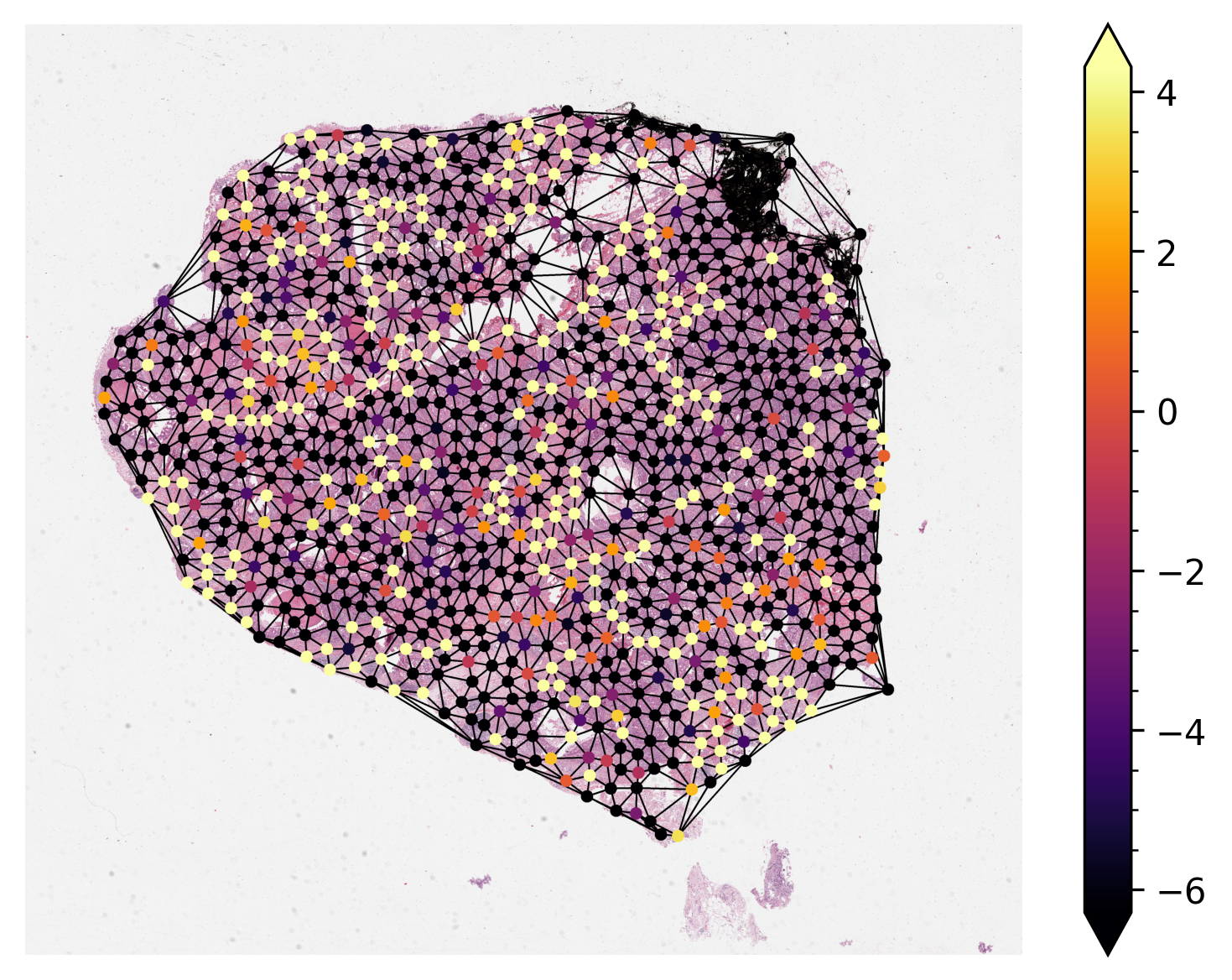
Visualize Node Activation of Graph Neural Network
Visualizing the activations of each node within the graph is sometimes necessary to either debug or verify the predictions of the graph neural network. Here, we demonstrate
Load pretrained model and run inference on one single sample graph.
Retrieve the node activations and plot them on the original WSI.
By default, notice that node activations are also output when running mode.forward(input) (or
simply model(input) in pytorch).
Most of the time the nodes within the graph will be at a different resolution
from the resolution at which we want to visualize them. Before plotting, we scale their coordinates
to the target resolution. We provide NODE_RESOLUTION and PLOT_RESOLUTION variables
respectively as the resolution of the node and the resolution to plot the graph.
NODE_SIZE = 25
NUM_NODE_FEATURES = 4
if USE_PRE_GENERATED:
    NODE_RESOLUTION = {"resolution": 0.5, "units": "mpp"}
else:
    NODE_RESOLUTION = {"resolution": 0.25, "units": "mpp"}
PLOT_RESOLUTION = {"resolution": 4.0, "units": "mpp"}
if FEATURE_MODE == "composition":
    cmap = plt.get_cmap("inferno")
    graph = graph.to("cpu")

    if USE_PRE_GENERATED:
        node_coordinates = np.array(graph.coords) / fx
    else:
        node_coordinates = np.array(graph.coordinates) / fx
    node_colors = (cmap(np.squeeze(node_activations))[..., :3] * 255).astype(np.uint8)
    edges = graph.edge_index.T

    thumb = reader.slide_thumbnail(**PLOT_RESOLUTION)
    thumb_overlaid = plot_graph(
        thumb.copy(),
        node_coordinates,
        edges,
        node_colors=node_colors,
        node_size=NODE_SIZE,
    )

    ax = plt.subplot(1, 1, 1)
    plt.imshow(thumb_overlaid)
    plt.axis("off")
    # Add minorticks on the colorbar to make it easy to read the
    # values off the colorbar.
    fig = plt.gcf()
    norm = mpl.colors.Normalize(
        vmin=np.min(node_activations),
        vmax=np.max(node_activations),
    )
    sm = plt.cm.ScalarMappable(cmap=cmap, norm=norm)
    cbar = fig.colorbar(sm, ax=ax, extend="both")
    cbar.minorticks_on()
    plt.show()