Patch extraction from Histology Images
Click to open in: [GitHub][Colab]
About this demo
In this example we will show how you can use tiatoolbox to extract patches from a large histology image. Tiatoolbox can extract patches in different ways, such as point-based, fixed-window, and variable-window patch extraction. One practical use of these tools is when using deep learning models that cannot accept large images in the input. In particular, we will introduce the use of our module
patchextraction (details).
Downloading the required files
We download, over the internet, a couple of files (a histology image and a csv file containing the positions of nuclei in that image). Download is needed once in each Colab session.
img_file_name = "sample_img.png"
csv_file_name = "sample_coordinates.csv"

# Downloading sample image from MoNuSeg
r = requests.get(
    "https://huggingface.co/datasets/TIACentre/TIAToolBox_Remote_Samples/resolve/main/testdata/patchextraction/TCGA-HE-7130-01Z-00-DX1.png",
    timeout=10,  # 10s
)
with Path(img_file_name).open("wb") as f:
    f.write(r.content)

# Downloading points list
r = requests.get(
    "https://huggingface.co/datasets/TIACentre/TIAToolBox_Remote_Samples/resolve/main/testdata/patchextraction/sample_patch_extraction.csv",
    timeout=10,  # 10s
)
with Path(csv_file_name).open("wb") as f:
    f.write(r.content)

logger.info("Download is complete.")
|2024-08-23|11:20:41.578| [INFO] Download is complete.
Reading image and annotation file
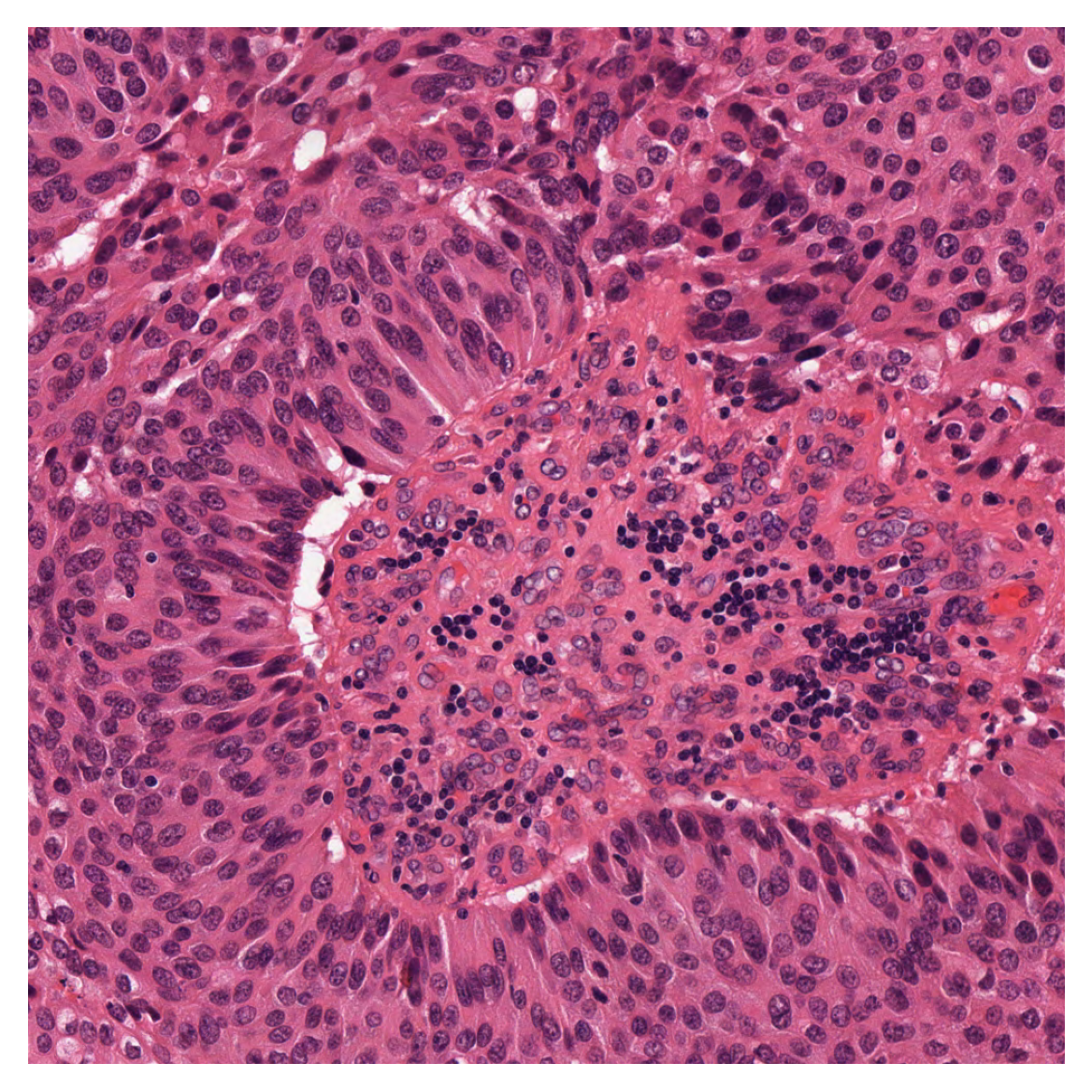
We use a sample image from the MoNuSeg dataset, for which nuclei have already been located (manually) and centroids computed. The sample image and list of points are loaded from the internet. The function read_locations returns a dataFrame, in which a typical row has the form $(x, y, class)$. Here $(x,y)$ are coordinates for a particular centroid, and class is the type of that patch. For this example, “class” can indicate the type of the nucleus, such as “epithelial” or “inflammatory”. In the simple situation we are illustrating here, biological information has not been provided, and is replaced by a meaningless number 0.0, which is just a place-holder. Dataframes in Python are handled using pandas. You don’t need to learn the details to understand this demo, but, if you want to use dataframes in your own code, or to replace data in this notebook by your own data, you will need to find out more about pandas.
input_img = imread(img_file_name)
centroids_list = read_locations(csv_file_name)

logger.info(
    "Image size: (%d, %d, %d)",
    input_img.shape[0],
    input_img.shape[1],
    input_img.shape[2],
)
logger.info("This image has %d point annotations", centroids_list.shape[0])
logger.info("\t" + centroids_list.head().to_string().replace("\n", "\n\t"))
|2024-08-23|11:20:41.866| [INFO] Image size: (1000, 1000, 3)
|2024-08-23|11:20:41.869| [INFO] This image has 1860 point annotations
|2024-08-23|11:20:41.897| [INFO] 	      x     y  class
	0  14.0   3.0    0.0
	1   3.0  15.0    0.0
	2  13.0  13.0    0.0
	3  58.0   8.0    0.0
	4  69.0   8.0    0.0
To see better what we are dealing with here, we show the image, first in its original form, and then with the desired centroids overlaid.
input_img = imread(img_file_name)
plt.imshow(input_img)
plt.axis("off")
plt.show()

# overlay nuclei centroids on image and plot
plt.imshow(input_img)
plt.scatter(np.array(centroids_list)[:, 0], np.array(centroids_list)[:, 1], s=1)
plt.axis("off")
plt.show()
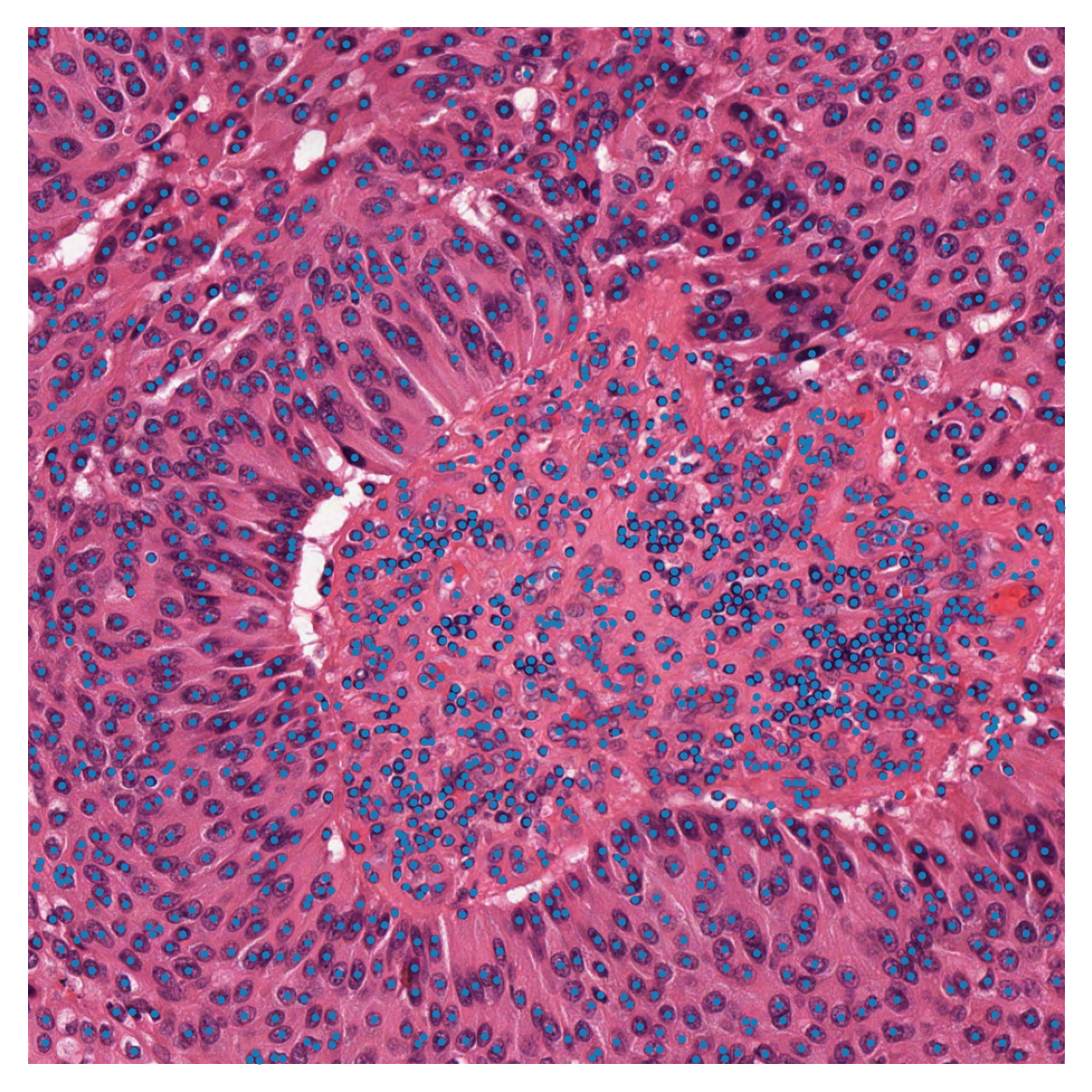
Patches based on point annotations
As you can see in the above figure, each nucleus is marked with a blue dot. To train a nucleus classifier computer program (or a beginning pathologist), it is helpful to see a nucleus in context, that is, within a surrounding patch. Therefore, we extract, for each nucleus, a patch centred on that nucleus. If the third column of our dataframe has been completed meaningfully (which is not the case in our example), it is then easy to save patches in different folders based on their biological significance or class=classification. This can be done using functions from the Python classes defined in our module patchextraction . (We are using both class=biological classification and class=Python class for coding.) The patch_extractor yields patches from the image, input_img, based on the centroids_list in a one-by-one manner. In the next code cell, we show how to use the function get_patch_extractor to obtain a suitable patch_extractor
patch_extractor = patchextraction.get_patch_extractor(
    input_img=input_img,  # input image path, numpy array, or WSI object
    locations_list=np.array(centroids_list)[
        500:600,
        :,
    ],  # path to list of points (csv, json), numpy list, panda DF
    method_name="point",  # also supports "slidingwindow"
    patch_size=(
        32,
        32,
    ),  # size of the patch to extract around the centroids from centroids_list
    resolution=0,
    units="level",
)
As you can see, patchextraction.get_patch_extractor accepts several arguments:
input_img: The image from which we want to extract patches. We can read the image and pass it to the function as a numpy array or instead, you can pass the path of the image file to the function.locations_list: The list of points at which the required patches will be centred. We load the points list as a panda data frame and pass it to the function or instead, you can pass to the function the path to a csv, npy or json file.method_name: This important argument specifies the type of patch extractor that we want to build. As we are looking to extract patches around centroid points, we use here thepointoption. Another option ofslidingwindowis also supported. Please refer to the documentation for more information.patch_size: Size of the patches.resolutionandunit: These arguments specify the level or micron-per-pixel resolution of the WSI. Here we specify the WSI’s level 0. In general, this is the level of the greatest resolution, although, in this particular case, the image has only one level. More information can be found in the documentation.
The patch_extractor yields information in small chunks, to avoid potential memory problems when the list of centroids is very long.
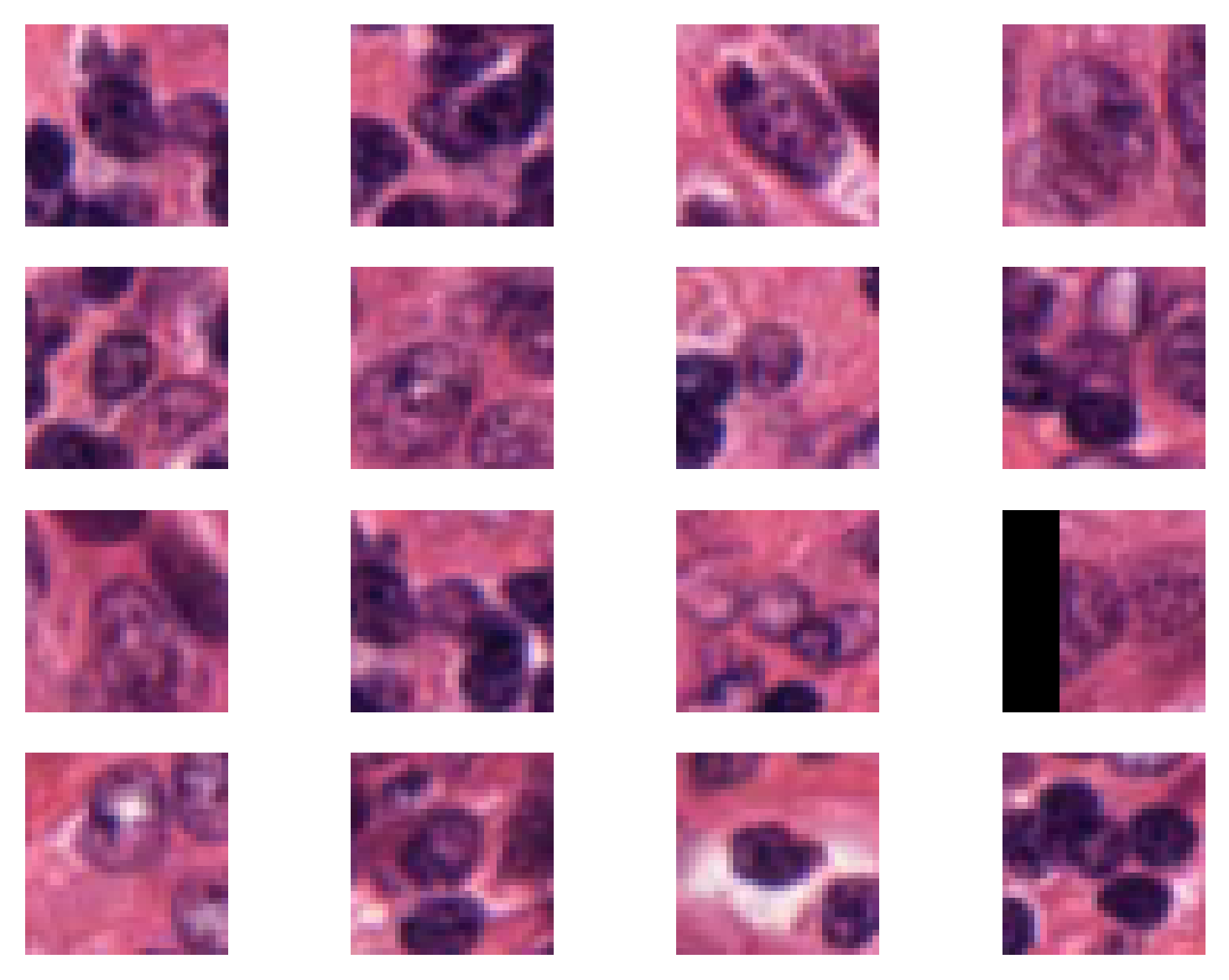
To extract patches using the patch_extractor we use for loops as below, where we extract the first 16 patches specified by centroids_list.
i = 1
# show only first 16 patches
num_patches_to_show = 16

for patch in patch_extractor:
    plt.subplot(4, 4, i)
    plt.imshow(patch)
    plt.axis("off")
    if i >= num_patches_to_show:
        break
    i += 1
plt.show()
|2024-08-23|11:20:49.363| [WARNING] Raw data is None.
|2024-08-23|11:20:49.387| [WARNING] Unknown scale (no objective_power or mpp)
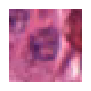
Using the defined point patch_extractor we can extract a patch around a particular point in the dataFrame. For that, you just simply specify the index of the desired point for the patch_extractor. For example, if we want to extract the patch around the 66th point in the dataFrame, we can do as below:
desired_patch = patch_extractor[66]

plt.subplot(4, 4, 1)
plt.imshow(desired_patch)
plt.axis("off")
(-0.5, 31.5, 31.5, -0.5)
Generate fixed-size patches
A very common practice in computational pathology, when analysing large histology images or WSIs, is to extract overlapping patches from that image and analyse them one by one. Deep Learning models often cannot accept large images due to memory limitations. We designed a tool in Tiatoolbox to ease the process of overlapping patch extraction for such goals.
The same patchextraction class supports another method that allows the user to extract all the patches from the input image in an efficient way, using just one line of code. In order to do that, one changes the method name in the patchextraction to "slidingwindow" as below:
fixed_patch_extractor = patchextraction.get_patch_extractor(
    input_img=input_img,  # input image path, numpy array, or WSI object
    method_name="slidingwindow",  # also supports "point" and "slidingwindow"
    patch_size=(
        500,
        500,
    ),  # size of the patch to extract around the centroids from centroids_list
    stride=(500, 500),  # stride of extracting patches, default is equal to patch_size
)
|2024-08-23|11:20:52.289| [WARNING] Raw data is None.
|2024-08-23|11:20:52.291| [WARNING] Unknown scale (no objective_power or mpp)
The patchextraction splits the input image into patches of size 500x500 without any overlap, because the stride of patch extraction is the same as patch_size. The fixed_patch_extractor is an iterator that yields a patch each time it is called. As in the example above, we can use a for loop to access these patches:
i = 1
for patch in fixed_patch_extractor:
    plt.subplot(2, 2, i)
    plt.imshow(patch)
    plt.axis("off")
    i += 1
plt.show()
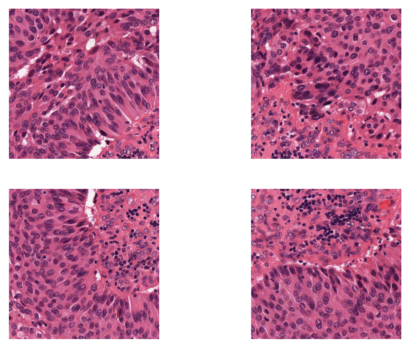
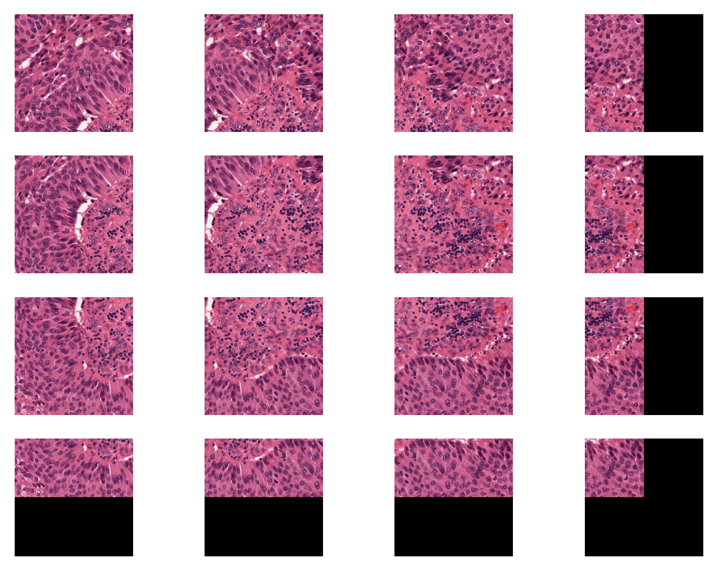
Otherwise, by setting the stride smaller than the ‘patch_size`, we can extract overlapping patches. Below we extract 500x500 patches that have 250 pixels overlap in both axes.
fixed_patch_extractor = patchextraction.get_patch_extractor(
    input_img=input_img,  # input image path, numpy array, or WSI object
    method_name="slidingwindow",  # also supports "point" and "slidingwindow"
    patch_size=(
        500,
        500,
    ),  # size of the patch to extract around the centroids from centroids_list
    stride=(250, 250),  # 250 pixels overlap in both axes
)

i = 1
for patch in fixed_patch_extractor:
    plt.subplot(4, 4, i)
    plt.imshow(patch)
    plt.axis("off")
    i += 1
plt.show()
|2024-08-23|11:20:54.458| [WARNING] Raw data is None.
|2024-08-23|11:20:54.467| [WARNING] Unknown scale (no objective_power or mpp)
Remember, you can always access a specific patch in your patch extractor using its index, as below:
patch_idx = 4  # setting the patch index to point the fifth (middle) patch
this_path = fixed_patch_extractor[patch_idx]  # extracting the desired patch

# displaying the patch
plt.subplot(3, 3, 1)
plt.imshow(this_path)
plt.axis("off")
plt.show()
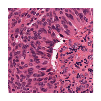
As you can see, the extracted patch is the same as the middle one in the above example.
Masked patch extraction
We can also do masked patch extraction. We often will not want to extract all the patches in an image. In the case of a WSI, we will often only want patches from the tissue region. Or, we may have more complex critera, and wish to extract patches only within certain annotated regions. We will demonstrate both these cases. Lets download a sample WSI and demonstrate this by extracting only patches that contain a significant amount of tissue.
# download a sample WSI. This may take a minute or 2 as it is a large file
from tiatoolbox.utils.misc import download_data
from tiatoolbox.wsicore import WSIReader

wsi_file_name = "sample_wsi.svs"
wsi_path = download_data(
    "https://huggingface.co/datasets/TIACentre/TIAToolBox_Remote_Samples/resolve/main/sample_wsis/TCGA-3L-AA1B-01Z-00-DX1.8923A151-A690-40B7-9E5A-FCBEDFC2394F.svs",
    wsi_file_name,
)
wsi = WSIReader.open(wsi_path)
In the next code block we will set up a patch extractor and have the tissue mask automatically generated from the wsi through a simple otsu threshold approach (for more details see (details)). We could also provide a manually generated mask if we preferred.
from tiatoolbox.tools.patchextraction import SlidingWindowPatchExtractor

extractor = SlidingWindowPatchExtractor(
    wsi_path,
    patch_size=(512, 512),
    stride=(512, 512),
    input_mask="otsu",
    min_mask_ratio=0.5,
)
|2024-08-23|11:21:57.148| [WARNING] Read: Scale > 1.This means that the desired resolution is higher than the WSI baseline (maximum encoded resolution). Interpolation of read regions may occur.
We will plot the slide thumbnail, the mask that has been auto-generated for us, and a scatter plot of the locations dataframe from which the extractor would provide patches, side-by-side
def plot_mask_and_locs(thumb: np.ndarray, mask: np.ndarray, locs: dict) -> None:
    """Plots slide thumbnail, mask and patch locations side by side."""
    _, axs = plt.subplots(1, 3)
    for ax in axs:
        ax.set(xticks=[], yticks=[])

    # Plot slide thumbnail
    axs[0].imshow(thumb)
    axs[0].set_title("Slide Thumbnail")

    # Plot mask
    axs[1].imshow(mask, cmap="gray")
    axs[1].set_title("Mask")

    # Plot scatter plot of locations (scales to thumb resolution)
    axs[2].scatter(
        locs["x"] * (1.25 / 40),
        locs["y"] * (1.25 / 40),
        s=0.1,
    )
    axs[2].set_title("Locations Scatter Plot")
    # make axes same as previous two plots
    axs[2].set_xlim(0, mask.shape[1])
    axs[2].set_ylim(mask.shape[0], 0)
    axs[2].set_aspect("equal", "box")

    # Display the plot
    plt.show()


plot_mask_and_locs(wsi.slide_thumbnail(), extractor.mask.img, extractor.locations_df)
|2024-08-23|11:21:58.626| [WARNING] Read: Scale > 1.This means that the desired resolution is higher than the WSI baseline (maximum encoded resolution). Interpolation of read regions may occur.

As we can see, the mask covers the tissue region, and we will extract patches only from within that mask.
We will now also download an annotation store of patch predictions. This annotation store is created using the tiatoolbox PatchPredictor (for more information see example notebook 5). The predictions are plotted below.
from tiatoolbox.data import _fetch_remote_sample
from tiatoolbox.wsicore.wsireader import AnnotationStoreReader

ann_path = _fetch_remote_sample("patch_annotations")  # download sample annotations
ann_reader = AnnotationStoreReader(ann_path, base_wsi=wsi_path)
thumb = ann_reader.slide_thumbnail(resolution=6, units="mpp")  # visualize them
plt.imshow(thumb)
ax = plt.gca()
ax.set_title("Patch predictions")
ax.set(xticks=[], yticks=[])
|2024-08-23|11:22:03.892| [WARNING] Query is not using an index. Consider adding an index to improve performance.
[[], []]

We can provide this annotation store to the patch extractor to be used as a mask, and provide a filter string to extract only patches that satisfy our filter. We will use it to extract patches only from the tumor region below.
extractor = SlidingWindowPatchExtractor(
    wsi_path,
    patch_size=(512, 512),
    stride=(512, 512),
    input_mask=str(ann_path),
    store_filter="props['type']=='TUM'",
    min_mask_ratio=0.5,
)

fig, axs = plt.subplots(1, 3)
for ax in axs:
    ax.set(xticks=[], yticks=[])

# Plot slide thumbnail
axs[0].imshow(wsi.slide_thumbnail())
axs[0].set_title("Slide Thumbnail")

# Plot mask
axs[1].imshow(extractor.mask.img, cmap="gray")
axs[1].set_title("Mask")

# Plot scatter plot of locations
axs[2].scatter(
    extractor.locations_df["x"] * (1.25 / 40),
    extractor.locations_df["y"] * (1.25 / 40),
    s=0.1,
)
axs[2].set_title("Locations Scatter Plot")

# make axes consistent
axs[2].set_xlim(0, extractor.mask.img.shape[1])
axs[2].set_ylim(extractor.mask.img.shape[0], 0)
axs[2].set_aspect("equal", "box")


# Display the plot
plt.show()
|2024-08-23|11:22:15.396| [WARNING] Read: Scale > 1.This means that the desired resolution is higher than the WSI baseline (maximum encoded resolution). Interpolation of read regions may occur.
|2024-08-23|11:22:16.254| [WARNING] Read: Scale > 1.This means that the desired resolution is higher than the WSI baseline (maximum encoded resolution). Interpolation of read regions may occur.

As we can see, the mask, and so the locations from which the extractor will provide patches, now covers only the tumor region. This provides a lot of flexibility to extract only the patches we need to complete a task.
Excercise: to get the above mask we used store_filter=”props[‘type’]==’TUM’” to get only tumor annotations, but any valid filter string on properties in the annotation store could be used instead (for more details see annotation store documentation). Try out some other filters, to get for example stroma patches instead. The property values in the annotation store can be explored using pquery, or using the visualization interface.
from tiatoolbox.annotation.storage import SQLiteStore

store = SQLiteStore(ann_path)
types = store.pquery("props['type']")
print(f"Unique values of 'type' in properties: {types}")  # noqa: T201
|2024-08-23|11:22:18.404| [WARNING] Query is not using an index. Consider adding an index to improve performance.
Unique values of 'type' in properties: {'MUS', 'ADI', 'TUM', 'NORM', 'LYM', 'DEB', 'BACK', 'STR', 'MUC'}