Masking tissue region in whole slide images

Click to open in: [GitHub][Colab]

About this demo

In this example, we will show how you can use tiatoolbox to easily find the tissue region in a whole slide image. Apart from tissue regions, WSIs usually show large blank (glass) background areas that contain no information. Therefore, it is essential to detect the informative (tissue) region in the WSI before any action (like patch extraction and classification). We call this step, “tissue masking”. In particular, we introduce the use of our module tissuemask (details) which distinguishes tissue from glass, using an automatic image thresholding algorithm (Otsu’s method) and some morphological operations.

Importing related libraries

We will start by importing some libraries required to run this notebook.

"""Import modules required to run the Jupyter notebook."""

from __future__ import annotations

from pathlib import Path
from typing import TYPE_CHECKING

import matplotlib as mpl
import matplotlib.pyplot as plt
import requests

if TYPE_CHECKING:
    import numpy as np

from tiatoolbox.tools.tissuemask import MorphologicalMasker
from tiatoolbox.wsicore.wsireader import WSIReader

mpl.rcParams["figure.dpi"] = 150  # for high resolution figure in notebook

Downloading the required files

The next cell creates a temporary directory tmp and downloads to that directory, from the internet, an image file. The code illustrates a standard programming technique, designed to minimize the harmful effects of “hard-coding” choices that a user might like to change. Our choices are made explicitly only once, to minimize the amount of editing needed by a user with different choices. The choices are encoded in python variables, in this case data_dir and sample_file_name, which do not need to be changed when the choices change, and which are used when repetition is needed.

If the notebook is run a second time, the tmp directory will be deleted (see above). Cleaning up, after a program is run, is easier when all temporary data is collected at a single point, in this case in the directory tmp.

data_dir = "./tmp"
sample_file_name = "sample_wsi_small.svs"

user_sample_wsi_path = None
if user_sample_wsi_path is None:
    sample_wsi_path = f"{data_dir}/{sample_file_name}"
else:
    sample_wsi_path = user_sample_wsi_path
if not Path(sample_wsi_path).exists():
    Path(data_dir).mkdir()
    r = requests.get(
        "https://tiatoolbox.dcs.warwick.ac.uk/sample_wsis/CMU-1-Small-Region.svs",
        timeout=60,  # 60s
    )
    with Path(sample_wsi_path).open("wb") as f:
        f.write(r.content)

Reading a WSI and its Thumbnail

The toolbox provides a common interface for different whole slide image file formats produced by different vendors. The functions WSIReader.open takes a file path to an image as input and returns an instance of the appropriate subclass of WSIReader. For more information about WSI reading in tiatoolbox, please refer to the documentation and the notebook example dedicated to this topic.

wsi = WSIReader.open(input_img=sample_wsi_path)
print(type(wsi))  # noqa: T201

<class 'tiatoolbox.wsicore.wsireader.OpenSlideWSIReader'>

From the output of the cell above, note that the python variable wsi does not refer to an unadorned WSI, but to a more complex object possessing a number of very useful class methods, enabling it to conveniently read various aspects of the image. First, let’s check the basic WSI information, such as magnification, dimension, etc. (mpp= microns per pixel).

wsi_info = wsi.info.as_dict()
# Print one item per line
print(*list(wsi_info.items()), sep="\n")  # noqa: T201

('objective_power', 20.0)
('slide_dimensions', (2220, 2967))
('level_count', 1)
('level_dimensions', ((2220, 2967),))
('level_downsamples', [1.0])
('vendor', 'aperio')
('mpp', (0.499, 0.499))
('file_path', PosixPath('tmp/sample_wsi_small.svs'))
('axes', 'YXS')

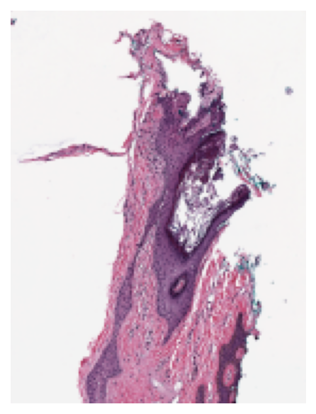
Working with tiatoolbox, it is easy to load a WSI thumbnail using the slide_thumbnail method of the wsi object. The thumbnail can be loaded with a different magnification, using a convenient choice of coordinates to indicate the resolution. The following options are available for the units argument:

• mpp: microns per pixel

• power: objective power (magnification)

• level: the level in the WSI pyramidal file

• baseline: pixels per baseline pixel. A baseline pixel is a pixel in the level (zero) of the greatest available magnification in this WSI.

We load and show the thumbnail at $\times1.25$ objective power as follows:

wsi_thumb = wsi.slide_thumbnail(resolution=1.25, units="power")
plt.imshow(wsi_thumb)
plt.axis("off")
plt.show()

Generating tissue mask in 1 line of code

The task is to distinguish between tissue and glass (no tissue) in the WSI. We compute a mask, by which we mean a binary colouring of the pixels to either blue=glass or yellow=tissue. Generating the tissue mask for a WSI using tiatoolbox is as simple as the following line of code:

mask = wsi.tissue_mask(resolution=1.25, units="power")

The two Python variables mask and wsi are both instances of the class WSIReader, and therefore have the same attributes, and can be treated in the same way. For example, we can visualize the original image and the mask next to each other at the same resolution and at the same size. Now, let’s see the thumbnails of the original wsi and its mask at the same resolution.

mask_thumb = mask.slide_thumbnail(
    resolution=1.25,
    units="power",
)  # extracting the mask_thumb at the same resolution as wsi_thumb


# showing the result
def show_side_by_side(image_1: np.ndarray, image_2: np.ndarray) -> None:
    """Helper function to shows images side-by-side."""
    plt.subplot(1, 2, 1)
    plt.imshow(image_1)
    plt.axis("off")
    plt.subplot(1, 2, 2)
    plt.imshow(image_2)
    plt.axis("off")
    plt.show()


show_side_by_side(wsi_thumb, mask_thumb)

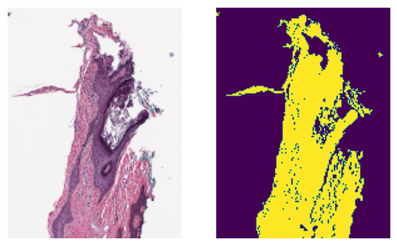
As you can see, the generated mask resembles the tissue area of the original WSI pretty closely. This kind of mask is usually used in digital pathology pipelines to specify the regions from which to extract patches at high resolution. Besides, extracting thumbnails, we can also extract regions from the mask object in the same way that we do for the wsi object:

wsi_region = wsi.read_region(location=(1024, 512), level=0, size=(512, 512))
mask_region = mask.read_region(location=(1024, 512), level=0, size=(512, 512))

show_side_by_side(wsi_region, mask_region)

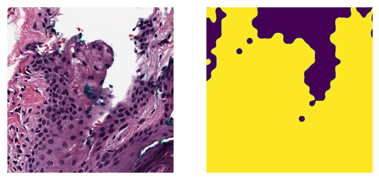
As expected, the coordinates of the original wsi and the mask line up precisely. This can be particularly useful if you want to calculate statistics of the tissue region in a patch (e.g., tissue area, intensity, and texture information).

There are some options (arguments) that can be used when calling tissue_mask() to achieve a more detailed tissue mask in high resolution or to remove small objects from the tissue mask. This will be explained in the next section.

Generating tissue masks for batch

Utilizing the functionalities in the tissuemask tool of the tiatoolbox, we can extract tissue masks for a batch of images. Here we use MorphologicalMasker to generate tissue masks for a list of input image regions.

First, we extract two different regions from the wsi. This is our batch of (only two) images to be processed using read_rect. We then instantiate a MorphologicalMasker object to be used in a later cell for extraction of masks from the batch:

# extracting the regions
mag_power = 20  # magnification power to extract patches and calculate the kernel_size
region1 = wsi.read_rect(
    location=(1024, 256),
    size=(512, 512),
    resolution=mag_power,
    units="power",
)
region2 = wsi.read_rect(
    location=(1536, 2048),
    size=(512, 512),
    resolution=mag_power,
    units="power",
)

# instantiating a MorphologicalMasker
masker = MorphologicalMasker(power=mag_power)

Now, let’s apply the masker on the extracted patches:

masks = masker.fit_transform([region1, region2])

# showing the results
show_side_by_side(region1, masks[0])
show_side_by_side(region2, masks[1])

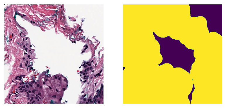
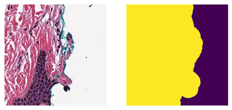
An optimal threshold is found by fit_transform using Otsu’s method. This is followed by deleting small objects and applying morphological dilation. Dilation results in overflow of the true boundaries of tissue regions. The overflow is deliberate, because we prefer not to miss tissue information.

The fit_transform function expects inputs that are (lists of) numpy arrays. That is why the inputs are enclosed by square brackets, eg masker.fit_transform([region1, region2]). The fit_transform function accepts a list of RGB images or a numpy array in the expected shape of N$\times$H$\times$W$\times$C (number of images, height, width, channels). It outputs a list of tissue masks

MorphologicalMasker can be used with different optional arguments:

• kernel_size: Size of the elliptical kernel to be used for morphological operations in mask post-processing.

• mpp: The microns per pixel of the image to be masked. Used to calculate kernel_size.

• power: The objective power of the image to be masked. Used to calculate kernel_size.

• min_region_size: Minimum region size in pixels to consider as foreground.

Note that only one of the named arguments kernel_size, mpp, or power should be used. Only the kernel_size is needed in morphological operations; the other two possible arguments are used only to calculate a suitable kernel_size. More information can be found in the definition of tissuemask.

Next we compute the mask of wsi_thumb using MorphologicalMasker and investigate the effect of changing parameters on the outputs:

def make_subplot(image: np.ndarray, title: str, k: int) -> None:
    """Make a 1x5 subplot."""
    plt.subplot(1, 5, k)
    plt.imshow(image)
    plt.axis("off")
    plt.title(title, fontdict={"fontsize": 5})


# default: kernel_size=1, min_region_size=1
masker = MorphologicalMasker()
masks_default = masker.fit_transform([wsi_thumb])

# meaning deleting objects smaller than 30 pixels in area
masker = MorphologicalMasker(min_region_size=30)
masks_small = masker.fit_transform([wsi_thumb])

# applying morphological dilation with a elliptical kernel (r=5) and
# deleting objects smaller than pi*5^2=78 pixels in area
masker = MorphologicalMasker(kernel_size=5)
masks_opt = masker.fit_transform([wsi_thumb])

# resulting to a over estimated kernel_size, hence bigger mask
masker = MorphologicalMasker(power=20)
masks_big = masker.fit_transform([wsi_thumb])

# showing the result
make_subplot(wsi_thumb, "Thumbnail", 1)
make_subplot(masks_default[0], "Default mask", 2)
make_subplot(masks_small[0], "Setting min_region_size=30", 3)
make_subplot(masks_opt[0], "Setting kernel_size=5", 4)
make_subplot(masks_big[0], "Setting power=20", 5)

plt.show()

As you can see, changing the parameters can change the resulting mask considerably. But don’t worry! Normally you don’t need to change or set anything when you are working with WSIs in tiatoolbox. Use the default arguments of functions—the toolbox will try to find the best parameters for your input WSI (as we did when we called mask = wsi.tissue_mask()).

Feel free to try these functionalities on your own data, or change the parameters to see how they can affect the output mask.