Stain Normalization

Click to open in: [GitHub][Colab]

Why normalize colour?

Pathologists usually find it easy to ignore features of a whole slide image (WSI) that are irrelevant from the point of view of diagnosis and treatment. However, this is not the case for computers. A standard hazard in digital pathology is that a computer program, developed using WSIs from one centre, gives much less impressive results when tried on WSIs from another centre. There are many factors contributing to such problems, among which are differences in colouring of WSIs from two different centres, even when the same standardised staining protocols are in force. These differences can be due to variation in slide scanners, the experience and skill of technicians, the quality and concentration of antigens, incubation time and temperature, etc, etc. Ideally, the same tissue specimens, stained in different laboratories, should give the same results, but this ideal appears to be unreachable. Stain normalization is a common pre-processing step, whose objective is to reduce to a minimum colour differences that have no significance in clinical practice. tiatoolbox makes a few different stain-normalization algorithms available to the user, and we demonstrate how to use them in this notebook.

About this demo

In this example, we will

1. Load a sample WSI.

2. Extract a square patch.

3. Stain-normalize the tile using various built-in methods.

4. Stain-normalize with a user-defined stain matrix.
   

During the above steps, we will be using functions from our stainnorm module here. This demo assumes some understanding of the functions in the wsireader module (for example by going through the demo here).

Importing related libraries

We start by importing some necessary modules.

"""Import modules required to run the Jupyter notebook."""

from __future__ import annotations

# Clear logger to use tiatoolbox.logger
import logging

if logging.getLogger().hasHandlers():
    logging.getLogger().handlers.clear()

from pathlib import Path

import matplotlib as mpl
import matplotlib.pyplot as plt
import requests
import skimage.color

from tiatoolbox import data, logger
from tiatoolbox.tools import stainnorm
from tiatoolbox.wsicore import wsireader

mpl.rcParams["figure.dpi"] = 150  # for high resolution figure in notebook

|2023-07-24|15:50:50.949| [INFO] NumExpr defaulting to 2 threads.

Downloading the required files

We load a small WSI, specified with the help of the path variable user_sample_wsi_path (default value None). Unless this None value is changed, the WSI is downloaded from the web, as seen in the code below, and saved with filename given by the variable sample_file_name in the directory given by data_dir. Data generated by the notebook is stored under data_dir, providing rapid local access.

data_dir = "./tmp"
sample_file_name = "sample_wsi_small.svs"

user_sample_wsi_path = None


def download(url_path: str, save_path: str | Path) -> None:
    """Download url_path to save_path."""
    r = requests.get(url_path, timeout=60)
    with Path(save_path).open("wb") as f:
        f.write(r.content)


user_sample_wsi_path = None

if user_sample_wsi_path is None:
    sample_wsi_path = f"{data_dir}/{sample_file_name}"
else:
    sample_wsi_path = user_sample_wsi_path
if not Path(sample_wsi_path).exists():
    Path(sample_wsi_path).parent.mkdir(parents=True)
    url_path = (
        " https://tiatoolbox.dcs.warwick.ac.uk/sample_wsis/CMU-1-Small-Region.svs"
    )
    download(url_path, sample_wsi_path)

logger.info("Download is complete.")

|2023-07-24|15:51:21.059| [INFO] Download is complete.

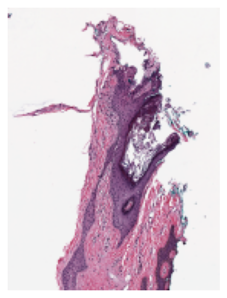
Reading in a WSI

It’s easy to read a WSI, and print important metadata. We plot a thumbnail version to find regions of interest.

# create a file handler
wsi_reader = wsireader.WSIReader.open(input_img=sample_wsi_path)
wsi_info = wsi_reader.info.as_dict()
# we will print out each info line by line
print(*list(wsi_info.items()), sep="\n")  # noqa: T201
wsi_thumb = wsi_reader.slide_thumbnail(resolution=1.25, units="power")

plt.imshow(wsi_thumb)
plt.axis("off")
plt.show()

('objective_power', 20.0)
('slide_dimensions', (2220, 2967))
('level_count', 1)
('level_dimensions', ((2220, 2967),))
('level_downsamples', [1.0])
('vendor', 'aperio')
('mpp', (0.499, 0.499))
('file_path', PosixPath('tmp/sample_wsi_small.svs'))
('axes', 'YXS')

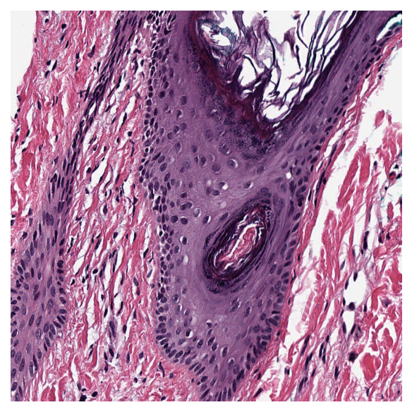
Extract a tile from the WSI

From the figure, a $50\times50$ patch with top-left at $[50,100]$ (XY-coordinate) in the thumbnail contains both stroma and gland tissue, and is therefore suitable for demonstrating different stainings. The thumbnail is loaded at $\times1.25$ objective power and the WSI at $\times20$. To convert to the highest resolution available, we multiply coordinates by $20/1.25 = 16$, obtaining a patch (named sample) with $800\times800$ pixels, and with the top-left corner of the patch at XY location $[800, 1600]$.

sample = wsi_reader.read_region(
    location=[800, 1600],
    level=0,
    size=[800, 800],  # in X, Y
)
plt.imshow(sample)
plt.axis("off")
plt.show()

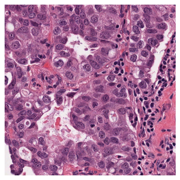
Stain normalizing a tile

We say that an image is a target, if we are trying to colour other images, of different tissue, consistently with the colouring of the target. We download a different image to act as target stain.

target_image = data.stain_norm_target()
plt.imshow(target_image)
plt.axis("off")
plt.show()

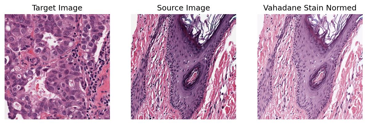
Vahadane method

We can stain-normalize the sample image to the target image using the widely known Vahadane method. The functionality of the normalizer is inspired by the sklearn calling style and is applied as follows:

stain_normalizer = stainnorm.VahadaneNormalizer()
stain_normalizer.fit(target_image)

normed_sample = stain_normalizer.transform(sample.copy())

plt.figure(figsize=(10, 5))
plt.subplot(1, 3, 1)
plt.imshow(target_image)
plt.title("Target Image")
plt.axis("off")
plt.subplot(1, 3, 2)
plt.imshow(sample)
plt.title("Source Image")
plt.axis("off")
plt.subplot(1, 3, 3)
plt.imshow(normed_sample)
plt.title("Vahadane Stain Normed")
plt.axis("off")
plt.show()

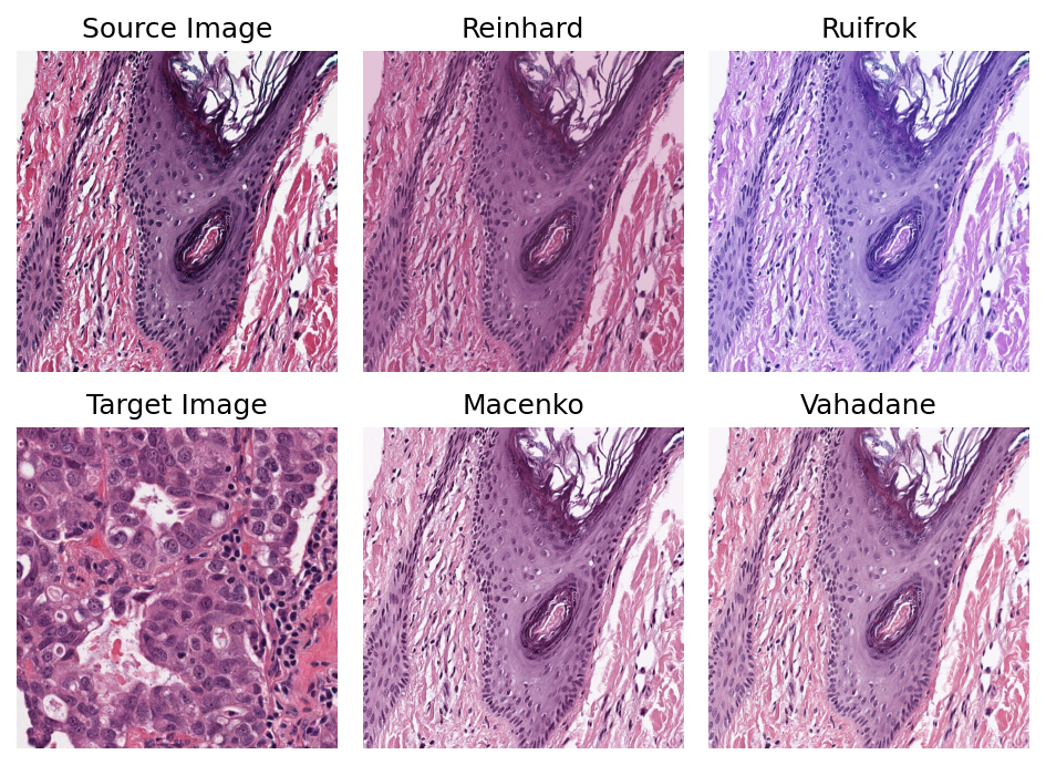
Other stain normalization methods

You can investigate one or more of the stain normalization methods we have implemented, by using either the class name as above, or our getter function get_normalizer. The getter function is applied to the corresponding method name. Below, we illustrate the latter approach. The stain normalization names are provided in the method_name_list variable. We sequentially apply each method on the sample image and plot them for visual comparison.

method_name_list = ["Reinhard", "Ruifrok", "Macenko", "Vahadane"]

plt.subplot(2, 3, 1)
plt.imshow(sample)
plt.title("Source Image")
plt.axis("off")
plt.subplot(2, 3, 4)
plt.imshow(target_image)
plt.title("Target Image")
plt.axis("off")

pos = [2, 3, 5, 6]
for idx, method_name in enumerate(method_name_list):
    stain_normalizer = stainnorm.get_normalizer(method_name)
    stain_normalizer.fit(target_image)

    normed_sample = stain_normalizer.transform(sample.copy())
    plt.subplot(2, 3, pos[idx])
    plt.imshow(normed_sample)
    plt.title(method_name.capitalize())
    plt.axis("off")
plt.tight_layout()
plt.show()

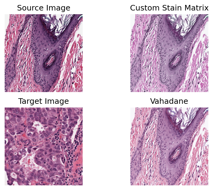
Custom staining

In addition to the four implemented methods, you can implement and use your own method. One way is to subclass the base class stainnorm.StainNormalizer. Another way is to provide your own custom stain conversion matrix as input to stainnorm.StainNormalizer.
(Note the former method is for advanced users only! In this notebook, we will only explore the customisation of the input stain matrix.)
As an example, we use a stain matrix available from the skimage library, namely Feulgen + Light Green, a colour model inspired by Robert Feulgen’s method of staining DNA. We finally compare using a custom defined stain matrix with using the Vahadane method.

stain_matrix = skimage.color.fgx_from_rgb[:2]
custom_normalizer = stainnorm.CustomNormalizer(stain_matrix)
custom_normalizer.fit(target_image)

vahadane_normalizer = stainnorm.VahadaneNormalizer()
vahadane_normalizer.fit(target_image)

normed_sample1 = custom_normalizer.transform(sample.copy())
normed_sample2 = stain_normalizer.transform(sample.copy())

plt.subplot(2, 2, 1)
plt.imshow(sample)
plt.title("Source Image")
plt.axis("off")
plt.subplot(2, 2, 3)
plt.imshow(target_image)
plt.title("Target Image")
plt.axis("off")
plt.subplot(2, 2, 2)
plt.imshow(normed_sample1)
plt.title("Custom Stain Matrix")
plt.axis("off")
plt.subplot(2, 2, 4)
plt.imshow(normed_sample2)
plt.title("Vahadane")
plt.axis("off")
plt.show()