Patch Prediction Models
Click to open in: [GitHub][Colab]
About this demo
In this example, we will show how to use TIAToolbox for patch-level prediction using a range of deep learning models. TIAToolbox can be used to make predictions on pre-extracted image patches or on larger image tiles / whole-slide images (WSIs), where image patches are extracted on the fly. WSI patch-level predictions can subsequently be aggregated to obtain a segmentation map. In particular, we will introduce the use of our module
patch_predictor (details). A full list of the available models trained and provided in TIAToolbox for patch-level prediction is given below.
Models trained on the Kather 100k dataset (details):
alexnet-kather100kresnet18-kather100kresnet34-kather100kresnet50-kather100kresnet101-kather100kresnext50_32x4d-kather100kresnext101_32x8d-kather100kwide_resnet50_2-kather100kwide_resnet101_2-kather100kdensenet121-kather100kdensenet161-kather100kdensenet169-kather100kdensenet201-kather100kmobilenet_v2-kather100kmobilenet_v3_large-kather100kmobilenet_v3_small-kather100kgooglenet-kather100k
Downloading the required files
We download, over the internet, image files used for the purpose of this notebook. In particular, we download a sample subset of validation patches that were used when training models on the Kather 100k dataset, a sample image tile and a sample whole-slide image. Downloading is needed once in each Colab session and it should take less than 1 minute. In Colab, if you click the file’s icon (see below) in the vertical toolbar on the left-hand side then you can see all the files which the code in this notebook can access. The data will appear here when it is downloaded.
img_file_name = global_save_dir / "sample_tile.png"
wsi_file_name = global_save_dir / "sample_wsi.svs"
patches_file_name = global_save_dir / "kather100k-validation-sample.zip"
imagenet_samples_name = global_save_dir / "imagenet_samples.zip"

logger.info("Download has started. Please wait...")

# Downloading sample image tile
download_data(
    "https://tiatoolbox.dcs.warwick.ac.uk/sample_imgs/CRC-Prim-HE-05_APPLICATION.tif",
    img_file_name,
)

# Downloading sample whole-slide image
download_data(
    "https://tiatoolbox.dcs.warwick.ac.uk/sample_wsis/TCGA-3L-AA1B-01Z-00-DX1.8923A151-A690-40B7-9E5A-FCBEDFC2394F.svs",
    wsi_file_name,
)

# Download a sample of the validation set used to train the Kather 100K dataset
download_data(
    "https://tiatoolbox.dcs.warwick.ac.uk/datasets/kather100k-validation-sample.zip",
    patches_file_name,
)
# Unzip it!
with ZipFile(patches_file_name, "r") as zipfile:
    zipfile.extractall(path=global_save_dir)

# Download some samples of imagenet to test the external models
download_data(
    "https://tiatoolbox.dcs.warwick.ac.uk/sample_imgs/imagenet_samples.zip",
    imagenet_samples_name,
)
# Unzip it!
with ZipFile(imagenet_samples_name, "r") as zipfile:
    zipfile.extractall(path=global_save_dir)

logger.info("Download is complete.")
Show code cell output
|2023-11-08|10:31:21.808| [INFO] Download has started. Please wait...
|2023-11-08|10:36:11.073| [INFO] Download is complete.
Get predictions for a set of patches
Below we use tiatoolbox to obtain the model predictions for a set of patches with a pretrained model.
We use patches from the validation subset of Kather 100k dataset. This dataset has already been downloaded in the download section above.
We first read the data and convert it to a suitable format. In particular, we create a list of patches and a list of corresponding labels.
For example, the first label in label_list will indicate the class of the first image patch in patch_list.
# read the patch data and create a list of patches and a list of corresponding labels

dataset_path = global_save_dir / "kather100k-validation-sample"

# set the path to the dataset
image_ext = ".tif"  # file extension of each image

# obtain the mapping between the label ID and the class name
label_dict = {
    "BACK": 0,
    "NORM": 1,
    "DEB": 2,
    "TUM": 3,
    "ADI": 4,
    "MUC": 5,
    "MUS": 6,
    "STR": 7,
    "LYM": 8,
}
class_names = list(label_dict.keys())
class_labels = list(label_dict.values())

# generate a list of patches and generate the label from the filename
patch_list = []
label_list = []
for class_name, label in label_dict.items():
    dataset_class_path = dataset_path / class_name
    patch_list_single_class = grab_files_from_dir(
        dataset_class_path,
        file_types="*" + image_ext,
    )
    patch_list.extend(patch_list_single_class)
    label_list.extend([label] * len(patch_list_single_class))


# show some dataset statistics
plt.bar(class_names, [label_list.count(label) for label in class_labels])
plt.xlabel("Patch types")
plt.ylabel("Number of patches")

# count the number of examples per class
for class_name, label in label_dict.items():
    logger.info(
        "Class ID: %d -- Class Name: %s -- Number of images: %d",
        label,
        class_name,
        label_list.count(label),
    )


# overall dataset statistics
logger.info("Total number of patches: %d", (len(patch_list)))
|2023-11-08|10:36:11.158| [INFO] Class ID: 0 -- Class Name: BACK -- Number of images: 211
|2023-11-08|10:36:11.159| [INFO] Class ID: 1 -- Class Name: NORM -- Number of images: 176
|2023-11-08|10:36:11.166| [INFO] Class ID: 2 -- Class Name: DEB -- Number of images: 230
|2023-11-08|10:36:11.167| [INFO] Class ID: 3 -- Class Name: TUM -- Number of images: 286
|2023-11-08|10:36:11.168| [INFO] Class ID: 4 -- Class Name: ADI -- Number of images: 208
|2023-11-08|10:36:11.169| [INFO] Class ID: 5 -- Class Name: MUC -- Number of images: 178
|2023-11-08|10:36:11.170| [INFO] Class ID: 6 -- Class Name: MUS -- Number of images: 270
|2023-11-08|10:36:11.173| [INFO] Class ID: 7 -- Class Name: STR -- Number of images: 209
|2023-11-08|10:36:11.175| [INFO] Class ID: 8 -- Class Name: LYM -- Number of images: 232
|2023-11-08|10:36:11.176| [INFO] Total number of patches: 2000
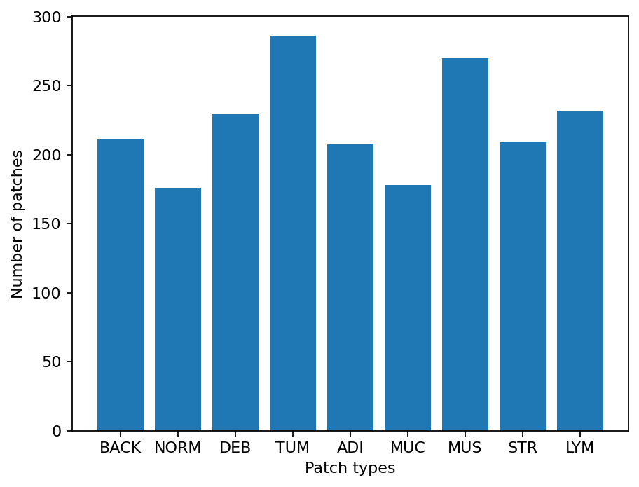
As you can see for this patch dataset, we have 9 classes/labels with IDs 0-8 and associated class names. describing the dominant tissue type in the patch:
BACK ⟶ Background (empty glass region)
LYM ⟶ Lymphocytes
NORM ⟶ Normal colon mucosa
DEB ⟶ Debris
MUS ⟶ Smooth muscle
STR ⟶ Cancer-associated stroma
ADI ⟶ Adipose
MUC ⟶ Mucus
TUM ⟶ Colorectal adenocarcinoma epithelium
It is easy to use this code for your dataset - just ensure that your dataset is arranged like this example (images of different classes are placed into different subfolders), and set the right image extension in the image_ext variable.
Predict patch labels in 2 lines of code
Now that we have the list of images, we can use TIAToolbox’s PatchPredictor to predict their category. First, we instantiate a predictor object and then we call the predict method to get the results.
predictor = PatchPredictor(pretrained_model="resnet18-kather100k", batch_size=32)
output = predictor.predict(imgs=patch_list, mode="patch", on_gpu=ON_GPU)
Show code cell output
Downloading: "https://download.pytorch.org/models/resnet18-f37072fd.pth" to /root/.cache/torch/hub/checkpoints/resnet18-f37072fd.pth
100%|██████████| 44.7M/44.7M [00:00<00:00, 146MB/s]
100%|###########################################| 63/63 [00:18<00:00,  3.40it/s]
Patch Prediction is Done!
The first line creates a CNN-based patch classifier instance based on the arguments and prepares a CNN model (generates the network, downloads pretrained weights, etc.). The CNN model used in this predictor can be defined using the pretrained_model argument. A complete list of supported pretrained classification models, that have been trained on the Kather 100K dataset, is reported in the first section of this notebook. PatchPredictor also enables you to use your own pretrained models for your specific classification application. In order to do that, you might need to change some input arguments for PatchPredictor, as we now explain:
model: Use an externally defined PyTorch model for prediction, with weights already loaded. This is useful when you want to use your own pretrained model on your own data. The only constraint is that the input model should followtiatoolbox.models.abc.ModelABCclass structure. For more information on this matter, please refer to our example notebook on advanced model techniques.pretrained_model: This argument has already been discussed above. With it, you can tell tiatoolbox to use one of its pretrained models for the prediction task. A complete list of pretrained models can be found here. If bothmodelandpretrained_modelarguments are used, thenpretrained_modelis ignored. In this example, we usedresnet18-kather100K,which means that the model architecture is an 18 layer ResNet, trained on the Kather100k dataset.pretrained_weight: When using apretrained_model, the corresponding pretrained weights will also be downloaded by default. You can override the default with your own set of weights via thepretrained_weightargument.batch_size: Number of images fed into the model each time. Higher values for this parameter require a larger (GPU) memory capacity.
The second line in the snippet above calls the predict method to apply the CNN on the input patches and get the results. Here are some important predict input arguments and their descriptions:
mode: Type of input to be processed. Choose frompatch,tileorwsiaccording to your application. In this first example, we predict the tissue type of histology patches, so we use thepatchoption. The use oftileandwsioptions are explained below.imgs: List of inputs. When usingpatchmode, the input must be a list of images OR a list of image file paths, OR a Numpy array corresponding to an image list. However, for thetileandwsimodes, theimgsargument should be a list of paths to the input tiles or WSIs.return_probabilities: set to True to get per class probabilities alongside predicted labels of input patches. If you wish to merge the predictions to generate prediction maps fortileorwsimodes, you can setreturn_probabilities=True.
In the patch prediction mode, the predict method returns an output dictionary that contains the predictions (predicted labels) and probabilities (probability that a certain patch belongs to a certain class).
The cell below uses common python tools to visualize the patch classification results in terms of classification accuracy and confusion matrix.
acc = accuracy_score(label_list, output["predictions"])
logger.info("Classification accuracy: %f", acc)

# Creating and visualizing the confusion matrix for patch classification results
conf = confusion_matrix(label_list, output["predictions"], normalize="true")
df_cm = pd.DataFrame(conf, index=class_names, columns=class_names)

# show confusion matrix
sns.heatmap(df_cm, cmap="Blues", annot=True, fmt=".0%")
plt.show()
|2023-11-08|10:36:34.474| [INFO] Classification accuracy: 0.993000
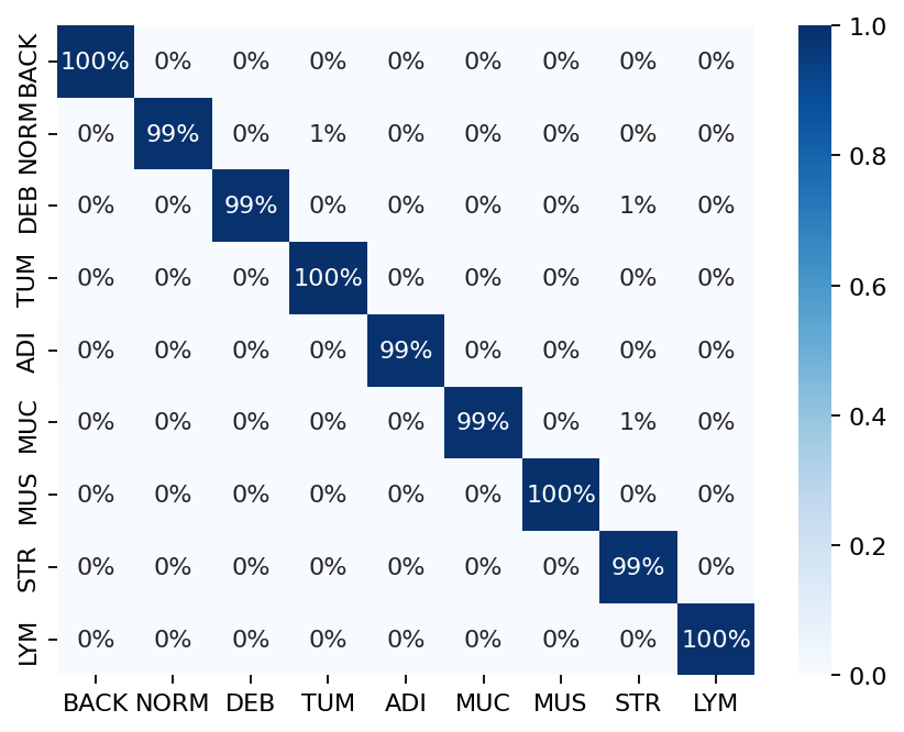
Try changing the pretrained_model argument when making PatchPredictor instant and see how it can affect the classification output accuracy.
Get predictions for patches within an image tile
We now demonstrate how to obtain patch-level predictions for a large image tile. It is quite a common practice in computational pathology to divide a large image into several patches (often overlapping) and then aggregate the results to generate a prediction map for different regions of the large image. As we are making a prediction per patch again, there is no need to instantiate a new PatchPredictor class. However, we should tune the predict input arguments to make them suitable for tile prediction. The predict function then automatically extracts patches from the large image tile and predicts the label for each of them. As the predict function can accept multiple tiles in the input to be processed and each input tile has potentially many patches, we save results in a file when more than one image is provided. This is done to avoid any problems with limited computer memory. However, if only one image is provided, the results will be returned as in patch mode.
Now, we try this function on a sample image tile. For this example, we use a tile that was released with the Kather et al. 2016 paper. It has been already downloaded in the Download section of this notebook.
Let’s take a look.
# reading and displaying a tile image
input_tile = imread(img_file_name)

plt.imshow(input_tile)
plt.axis("off")
plt.show()

logger.info(
    "Tile size is: (%d, %d, %d)",
    input_tile.shape[0],
    input_tile.shape[1],
    input_tile.shape[2],
)
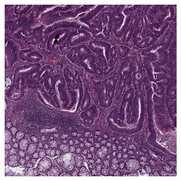
|2023-11-08|10:36:40.768| [INFO] Tile size is: (5000, 5000, 3)
Patch-level prediction in 2 lines of code for big histology tiles
As you can see, the size of the tile image is 5000x5000 pixels. This is quite big and might result in computer memory problems if fed directly into a deep learning model. However, the predict method of PatchPredictor handles this big tile seamlessly by processing small patches independently. You only need to change the mode argument to tile and a couple of other arguments, as explained below.
rmdir(global_save_dir / "tile_predictions")
img_file_name = Path(img_file_name)

predictor = PatchPredictor(pretrained_model="resnet18-kather100k", batch_size=32)
tile_output = predictor.predict(
    imgs=[img_file_name],
    mode="tile",
    merge_predictions=True,
    patch_input_shape=[224, 224],
    stride_shape=[224, 224],
    resolution=1,
    units="baseline",
    return_probabilities=True,
    save_dir=global_save_dir / "tile_predictions",
    on_gpu=ON_GPU,
)
Show code cell output
|2023-11-08|10:36:41.188| [WARNING] WSIPatchDataset only reads image tile at `units="baseline"`. Resolutions will be converted to baseline value.
|2023-11-08|10:36:41.191| [WARNING] WSIPatchDataset only reads image tile at `units="baseline"` and `resolution=1.0`.
|2023-11-08|10:36:42.083| [WARNING] Raw data is None.
100%|###########################################| 17/17 [00:02<00:00,  6.49it/s]
|2023-11-08|10:36:45.458| [WARNING] Image is not pyramidal hence read is forced to be at `units='baseline'` and `resolution=1.0`.
|2023-11-08|10:36:45.459| [WARNING] Raw data is None.
|2023-11-08|10:36:45.464| [WARNING] Unknown scale (no objective_power or mpp)
The new arguments in the input of predict method are:
mode='tile': the type of image input. We usetilesince our input is a large image tile.imgs: in tile mode, the input is required to be a list of file paths.save_dir: Output directory when processing multiple tiles. We explained before why this is necessary when we are working with multiple big tiles.patch_size: This parameter sets the size of patches (in [W, H] format) to be extracted from the input files, and for which labels will be predicted.stride_size: The stride (in [W, H] format) to consider when extracting patches from the tile. Using a stride smaller than the patch size results in overlapping between consecutive patches.labels(optional): List of labels with the same size asimgsthat refers to the label of each input tile (not to be confused with the prediction of each patch).
In this example, we input only one tile. Therefore the toolbox does not save the output as files and instead returns a list that contains an output dictionary with the following keys:
coordinates: List of coordinates of extracted patches in the following format:[x_min, y_min, x_max, y_max]. These coordinates can be used to later extract the same region from the input tile/WSI or regenerate a prediction map based on thepredictionlabels for each patchpredictions: List of predicted labels for each of the tile’s patches.label: Label of the tile generalized to each patch.
Keep in mind that if we had several items in the imgs input, then the result would be saved in JSON format to the specified save_dir and the returned output will be a list of paths to each of the saved JSON files
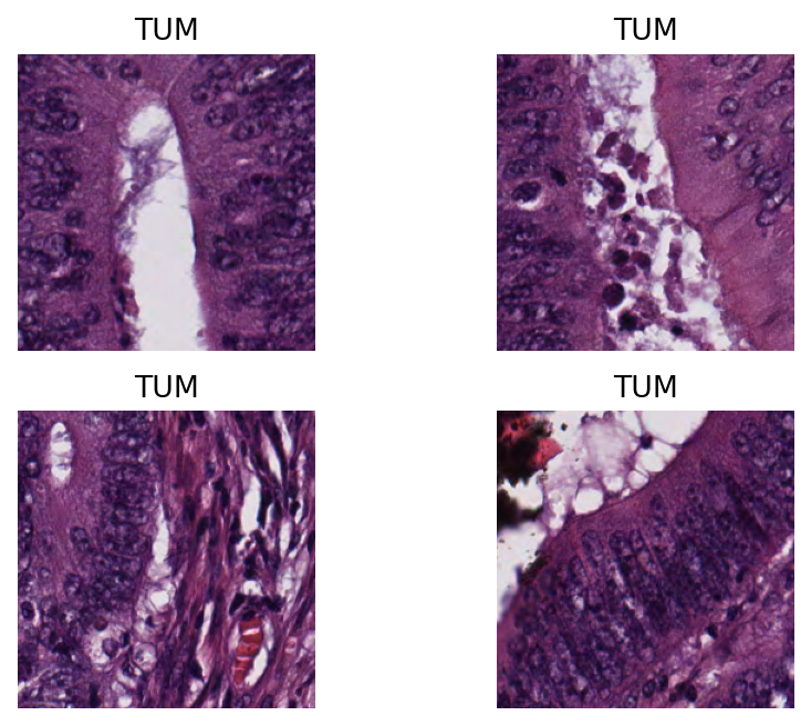
Now, we visualize some patch-level results.
Visualisation of tile results
Below we will show some of the results generated by our patch-level predictor on the input image tile. First, we will show some individual patch predictions and then we will show the merged patch level results on the entire image tile.
# individual patch predictions sampled from the image tile

# extract the information from output dictionary
coordinates = tile_output[0]["coordinates"]
predictions = tile_output[0]["predictions"]

# select 4 random indices (patches)
rng = np.random.default_rng()  # Numpy Random Generator
random_idx = rng.integers(0, len(predictions), (4,))

for i, idx in enumerate(random_idx):
    this_coord = coordinates[idx]
    this_prediction = predictions[idx]
    this_class = class_names[this_prediction]

    this_patch = input_tile[
        this_coord[1] : this_coord[3],
        this_coord[0] : this_coord[2],
    ]
    plt.subplot(2, 2, i + 1), plt.imshow(this_patch)
    plt.axis("off")
    plt.title(this_class)
Here, we show a prediction map where each colour denotes a different predicted category. We overlay the prediction map on the original image. To generate this prediction map, we utilize the merge_predictions method from the PatchPredictor class which accepts as arguments the path of the original image, predictor outputs, mode (set to tile or wsi), tile_resolution (at which tiles were originally extracted) and resolution (at which the prediction map is generated), and outputs the “Prediction map”, in which regions have indexed values based on their classes.
To visualize the prediction map as an overlay on the input image, we use the overlay_prediction_mask function from the tiatoolbox.utils.visualization module. It accepts as arguments the original image, the prediction map, the alpha parameter which specifies the blending ratio of overlay and original image, and the label_info dictionary which contains names and desired colours for different classes. Below we generate an example of an acceptable label_info dictionary and show how it can be used with overlay_patch_prediction.
# visualization of merged image tile patch-level prediction.

tile_output[0]["resolution"] = 1.0
tile_output[0]["units"] = "baseline"

label_color_dict = {}
label_color_dict[0] = ("empty", (0, 0, 0))
colors = cm.get_cmap("Set1").colors
for class_name, label in label_dict.items():
    label_color_dict[label + 1] = (class_name, 255 * np.array(colors[label]))
pred_map = predictor.merge_predictions(
    img_file_name,
    tile_output[0],
    resolution=1,
    units="baseline",
)
overlay = overlay_prediction_mask(
    input_tile,
    pred_map,
    alpha=0.5,
    label_info=label_color_dict,
    return_ax=True,
)
plt.show()
|2023-11-08|10:36:51.889| [WARNING] Image is not pyramidal hence read is forced to be at `units='baseline'` and `resolution=1.0`.
|2023-11-08|10:36:51.891| [WARNING] Raw data is None.
|2023-11-08|10:36:51.893| [WARNING] Unknown scale (no objective_power or mpp)
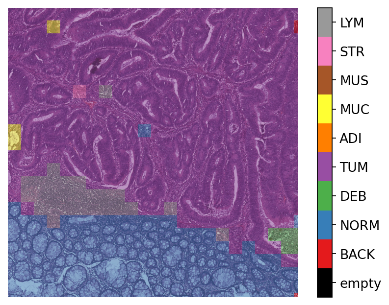
Note that overlay_prediction_mask returns a figure handler, so that plt.show() or plt.savefig() shows or, respectively, saves the overlay figure generated. Now go back and predict with a different stride_size or pretrained_model to see what effect this has on the output.
Get predictions for patches within a WSI
We demonstrate how to obtain predictions for all patches within a whole-slide image. As in previous sections, we will use PatchPredictor and its predict method, but this time we set the mode to 'wsi'. We also introduce IOPatchPredictorConfig, a class that specifies the configuration of image reading and prediction writing for the model prediction engine.
wsi_ioconfig = IOPatchPredictorConfig(
    input_resolutions=[{"units": "mpp", "resolution": 0.5}],
    patch_input_shape=[224, 224],
    stride_shape=[224, 224],
)
Parameters of IOPatchPredictorConfig have self-explanatory names, but let’s have look at their definition:
input_resolutions: a list specifying the resolution of each input head of model in the form of a dictionary. List elements must be in the same order as targetmodel.forward(). Of course, if your model accepts only one input, you just need to put one dictionary specifying'units'and'resolution'. But it’s good to know that TIAToolbox supports a model with more than one input.patch_input_shape: Shape of the largest input in (height, width) format.stride_shape: the size of stride (steps) between two consecutive patches, used in the patch extraction process. If the user setsstride_shapeequal topatch_input_shape, patches will be extracted and processed without any overlap.
Now that we have set everything, we try our patch predictor on a WSI. Here, we use a large WSI and therefore the patch extraction and prediction processes may take some time (make sure to set the ON_GPU=True if you have access to Cuda enabled GPU and Pytorch+Cuda).
predictor = PatchPredictor(pretrained_model="resnet18-kather100k", batch_size=64)
wsi_output = predictor.predict(
    imgs=[wsi_file_name],
    masks=None,
    mode="wsi",
    merge_predictions=False,
    ioconfig=wsi_ioconfig,
    return_probabilities=True,
    save_dir=global_save_dir / "wsi_predictions",
    on_gpu=ON_GPU,
)
Show code cell output
|2023-11-08|10:37:01.460| [WARNING] Read: Scale > 1.This means that the desired resolution is higher than the WSI baseline (maximum encoded resolution). Interpolation of read regions may occur.
100%|#########################################| 315/315 [05:18<00:00,  1.01s/it]
We introduce some new arguments for predict method:
mode: set to ‘wsi’ when analysing whole slide images.ioconfig: set the IO configuration information using theIOPatchPredictorConfigclass.resolutionandunit(not shown above): These arguments specify the level or micron-per-pixel resolution of the WSI levels from which we plan to extract patches and can be used instead ofioconfig. Here we specify the WSI’s level as'baseline', which is equivalent to level 0. In general, this is the level of greatest resolution. In this particular case, the image has only one level. More information can be found in the documentation.masks: A list of paths corresponding to the masks of WSIs in theimgslist. These masks specify the regions in the original WSIs from which we want to extract patches. If the mask of a particular WSI is specified asNone, then the labels for all patches of that WSI (even background regions) would be predicted. This could cause unnecessary computation.merge_predictions: You can set this parameter toTrueif you wish to generate a 2D map of patch classification results. However, for big WSIs you might need a large amount of memory available to do this on the file. An alternative (default) solution is to setmerge_predictions=False, and then generate the 2D prediction maps usingmerge_predictionsfunction as you will see later on.
We see how the prediction model works on our whole-slide images by visualizing the wsi_output. We first need to merge patch prediction outputs and then visualize them as an overlay on the original image. As before, the merge_predictions method is used to merge the patch predictions. Here we set the parameters resolution=1.25, units='power' to generate the prediction map at 1.25x magnification. If you would like to have higher/lower resolution (bigger/smaller) prediction maps, you need to change these parameters accordingly. When the predictions are merged, use the overlay_patch_prediction function to overlay the prediction map on the WSI thumbnail, which should be extracted at the same resolution used for prediction merging. Below you can see the result:
# visualization of whole-slide image patch-level prediction
overview_resolution = (
    4  # the resolution in which we desire to merge and visualize the patch predictions
)

# the unit of the `resolution` parameter. Can be "power", "level", "mpp", or "baseline"
overview_unit = "mpp"
wsi = WSIReader.open(wsi_file_name)
wsi_overview = wsi.slide_thumbnail(resolution=overview_resolution, units=overview_unit)
plt.figure(), plt.imshow(wsi_overview)
plt.axis("off")

pred_map = predictor.merge_predictions(
    wsi_file_name,
    wsi_output[0],
    resolution=overview_resolution,
    units=overview_unit,
)
overlay = overlay_prediction_mask(
    wsi_overview,
    pred_map,
    alpha=0.5,
    label_info=label_color_dict,
    return_ax=True,
)
plt.show()
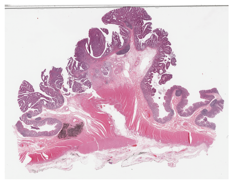
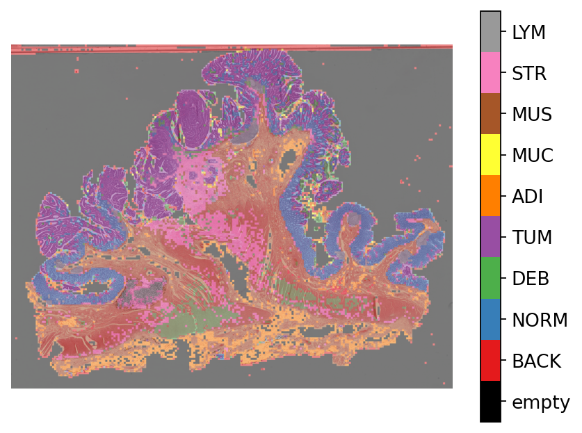
In this notebook, we show how we can use the PatchPredictor class and its predict method to predict the label for patches of big tiles and WSIs. We introduce merge_predictions and overlay_prediction_mask helper functions that merge the patch prediction outputs and visualize the resulting prediction map as an overlay on the input image/WSI.
All the processes take place within TIAToolbox and you can easily put the pieces together, following our example code. Just make sure to set inputs and options correctly. We encourage you to further investigate the effect on the prediction output of changing predict function parameters. Furthermore, if you want to use your own pretrained model for patch classification in the TIAToolbox framework (even if the model structure is not defined in the TIAToolbox model class), you can follow the instructions in our example notebook on advanced model techniques to gain some insights and guidance.