Slide Graph Full-pipeline Notebook

Click to open in: [GitHub]

About this notebook

This notebook is computationally intensive. We advise users to run this notebook locally on a machine with GPUs. To run the notebook on your local machine, set up your Python environment, as explained in the README file. You can edit the notebook during the session, for example substituting your own image files for the image files used in this demo. Experiment by changing the parameters of functions.

Introduction

This notebook is aimed at advanced users who are interested in using TIAToolbox as part of an experiment or larger project. Here we replicate the method in “SlideGraph+: Whole Slide Image Level Graphs to Predict HER2Status in Breast Cancer” by Lu et al. (2021) to generate a graph on the whole slide image level and directly predict a slide level label. Our task is to classify a whole slide image (WSI) as either HER2 negative or positive. For this work, we will use the TCGA-BRCA dataset.

Throughout this notebook we use modules from TIAToolbox to assist with common tasks including:

• Patch extraction

• Stain normalization

• Cell segmentation & classification

• Extraction of deep features

Note: Although the original paper was evaluated for HER2, the method itself can be applied to other mutation predictions. We provide a pretrained model for predicting ER (Estrogen receptor) status here (model weights) and here (model auxiliary). You can get the pre-generated graphs here and its node preprocessing model here. For predicting ER status, we use deep features coming from ResNet50 rather than the cellular structure.

%%bash
pip install -U numpy
pip install umap-learn ujson
pip uninstall -y torch-scatter torch-sparse torch-geometric
pip uninstall -y torch
pip install torch==1.10.0+cu113 torchvision==0.11.1+cu113 torchaudio==0.10.0+cu113 -f https://download.pytorch.org/whl/cu113/torch_stable.html
pip install torch-scatter -f https://data.pyg.org/whl/torch-1.10.0+cu113.html
pip install torch-sparse -f https://data.pyg.org/whl/torch-1.10.0+cu113.html
pip install torch-geometric

Preparation: Imports, Helpers, & Data Split

We begin by importing some libraries, defining some helper functions and defining the split of the dataset into train, validation, and test subsets.

Import Libraries

"""Import modules required to run the Jupyter notebook."""

from __future__ import annotations

# Clear logger to use tiatoolbox.logger
import logging

if logging.getLogger().hasHandlers():
    logging.getLogger().handlers.clear()

import copy
import os
import random
import shutil
import warnings
from collections import OrderedDict
from pathlib import Path
from typing import TYPE_CHECKING, Callable

# Third party imports
import joblib
import matplotlib as mpl
import matplotlib.pyplot as plt
import numpy as np
import pandas as pd
import torch
import torch.nn.functional as F  # noqa: N812

# Use ujson as replacement for default json because it's faster for large JSON
import ujson as json
from shapely.geometry import box as shapely_box
from shapely.strtree import STRtree
from skimage.exposure import equalize_hist
from sklearn.decomposition import PCA
from sklearn.linear_model import LogisticRegression as PlattScaling
from sklearn.metrics import average_precision_score as auprc_scorer
from sklearn.metrics import roc_auc_score as auroc_scorer
from sklearn.model_selection import StratifiedKFold, StratifiedShuffleSplit
from sklearn.preprocessing import StandardScaler
from torch import nn
from torch.nn import BatchNorm1d, Linear, ReLU
from torch.utils.data import Sampler
from torch_geometric.data import Batch, Data, Dataset
from torch_geometric.loader import DataLoader
from torch_geometric.nn import (
    EdgeConv,
    GINConv,
    global_add_pool,
    global_max_pool,
    global_mean_pool,
)
from tqdm import tqdm

from tiatoolbox import logger
from tiatoolbox.data import stain_norm_target
from tiatoolbox.models import (
    DeepFeatureExtractor,
    IOSegmentorConfig,
    NucleusInstanceSegmentor,
)
from tiatoolbox.models.architecture.vanilla import CNNBackbone
from tiatoolbox.tools.graph import SlideGraphConstructor
from tiatoolbox.tools.patchextraction import PatchExtractor
from tiatoolbox.tools.stainnorm import get_normalizer

# ! save_yaml, save_as_json => need same name, need to factor out jsonify
from tiatoolbox.utils.misc import download_data, save_as_json
from tiatoolbox.utils.visualization import plot_graph
from tiatoolbox.wsicore.wsireader import (
    OpenSlideWSIReader,
    Resolution,
    Units,
    WSIReader,
)

if TYPE_CHECKING:  # pragma: no cover
    from collections.abc import Iterator

warnings.filterwarnings("ignore")
mpl.rcParams["figure.dpi"] = 300  # for high resolution figure in notebook

GPU or CPU runtime

Processes in this notebook can be accelerated by using a GPU. Therefore, whether you are running this notebook on your system or Colab, you need to check and specify appropriate device e.g., “cuda” or “cpu” whether you are using GPU or CPU. In Colab, you need to make sure that the runtime type is set to GPU in the “Runtime→Change runtime type→Hardware accelerator”. If you are not using GPU, consider changing the device flag to cpu value, otherwise, some errors will be raised when running the following cells.

device = "cuda"  # Choose appropriate device

Helper Functions

Here we define some helper functions that will be used throughout the notebook:

def load_json(path: Path) -> dict | list | int | float | str:
    """Load JSON from a file path."""
    with path.open() as fptr:
        return json.load(fptr)


def rmdir(dir_path: Path) -> None:
    """Remove a directory."""
    if dir_path.is_dir():
        shutil.rmtree(dir_path)


def rm_n_mkdir(dir_path: Path) -> None:
    """Remove then re-create a directory."""
    if dir_path.is_dir():
        shutil.rmtree(dir_path)
    dir_path.mkdir(parents=True)


def mkdir(dir_path: Path) -> None:
    """Create a directory if it does not exist."""
    if not dir_path.is_dir():
        dir_path.mkdir(parents=True)


def recur_find_ext(root_dir: Path, exts: list[str]) -> list[str]:
    """Recursively find files with an extension in `exts`.

    This is much faster than glob if the folder
    hierachy is complicated and contain > 1000 files.

    Args:
        root_dir (Path):
            Root directory for searching.
        exts (list):
            List of extensions to match.

    Returns:
        List of full paths with matched extension in sorted order.

    """
    assert isinstance(exts, list)  # noqa: S101
    file_path_list = []
    for cur_path, _dir_list, file_list in os.walk(root_dir):
        for file_name in file_list:
            file_ext = Path(file_name).suffix
            if file_ext in exts:
                full_path = cur_path / file_name
                file_path_list.append(full_path)
    file_path_list.sort()
    return file_path_list

Loading The Dataset

For this dataset (TCGA-BRCA), the HER2 status is provided per patient instead of per slide. Therefore, we assign the same label to all WSIs coming from the same patient. WSIs that do not have labels are excluded from subsequent processing.

We begin this notebook with loading the data by doing the following:

1. Load a list of WSIs and associated tissue masks (file paths).

2. Convert the clinical infomation in .csv to labels.

3. Assign the patient label to each WSI

4. Filter out WSIs which do not have a label.

We use the following global variables:

• CLINICAL_FILE: The .csv file which contains the patient code and the associated labels.

• ROOT_OUTPUT_DIR: Root directory to save output under.

• WSI_DIR: Directory containing WSIs.

• MSK_DIR: Directory containing the corresponding WSI mask. If set to None, the subsequent process will use the default method in the toolbox to obtain the mask (via WSIReader.tissue_mask). Each mask file is assumed to be .png and any non-zero pixels within it are considered for processing.

By the end of this process, we obtain the following variables for subsequent operations

• wsi_paths: A list of file paths to WSIs.

• wsi_names: A list of WSI names in wsi_paths.

• msk_paths: A list of paths pointing to masks of each WSI in wsi_paths.

• label_df: A panda dataframe containing two columns: WSI-CODE and LABEL. Each row in the dataframe is a pair, whose first entry is the name of a WSI in the list wsi_names and whose second entry is the label of that WSI.

SEED = 5
random.seed(SEED)
rng = np.random.default_rng(SEED)
torch.manual_seed(SEED)
torch.cuda.manual_seed(SEED)

# Set these variables to run next cell either
# seperately or with customized parameters
ROOT_OUTPUT_DIR = Path("PATH/TO/DIR/")
WSI_DIR = Path("PATH/TO/DIR/")
MSK_DIR = None
CLINICAL_FILE = Path("PATH/TO/DIR/")

# * Query for paths

wsi_paths = recur_find_ext(WSI_DIR, [".svs", ".ndpi"])
wsi_names = [Path(v).stem for v in wsi_paths]
msk_paths = None if MSK_DIR is None else [f"{MSK_DIR}/{v}.png" for v in wsi_names]
assert len(wsi_paths) > 0, "No files found."  # noqa: S101

# * Generate WSI labels
clinical_df = pd.read_csv(CLINICAL_FILE)
patient_uids = clinical_df["PATIENT"].to_numpy()
patient_labels = clinical_df["HER2FinalStatus"].to_numpy()

patient_labels_ = np.full_like(patient_labels, -1)
patient_labels_[patient_labels == "Positive"] = 1
patient_labels_[patient_labels == "Negative"] = 0
sel = patient_labels_ >= 0

patient_uids = patient_uids[sel]
patient_labels = patient_labels_[sel]
assert len(patient_uids) == len(patient_labels)  # noqa: S101
clinical_info = OrderedDict(list(zip(patient_uids, patient_labels)))

# Retrieve patient code of each WSI, this is based on TCGA barcodes:
# https://docs.gdc.cancer.gov/Encyclopedia/pages/TCGA_Barcode/
wsi_patient_codes = np.array(["-".join(v.split("-")[:3]) for v in wsi_names])
wsi_labels = np.array(
    [clinical_info.get(v, np.nan) for v in wsi_patient_codes],
)

# * Filter the WSIs and paths that do not have labels
sel = ~np.isnan(wsi_labels)
# Simple sanity checks before filtering
assert len(wsi_paths) == len(wsi_names)  # noqa: S101
assert len(wsi_paths) == len(wsi_labels)  # noqa: S101
wsi_paths = np.array(wsi_paths)[sel]
wsi_names = np.array(wsi_names)[sel]
wsi_labels = np.array(wsi_labels)[sel]

label_df = list(zip(wsi_names, wsi_labels))
label_df = pd.DataFrame(label_df, columns=["WSI-CODE", "LABEL"])

Generate the Data Split

Now, we split our dataset into disjoint train, validation, and test subsets.

To that end, we define a new function called stratified_split. It receives:

• paired input of the samples and their labels

• the train, valid, and test percentages

and then returns a number of stratified splits.

Stratification means that, for each label, the proportion of samples with that label is as similar as possible in each of the three splits. Stratification ensures that any bias that might result from a particular label operates as equally as possible in each split. This is a standard way of avoiding bias due to possible confounding factors – here each label is regarded as a possible confounding factor.

def stratified_split(
    x: list,
    y: list,
    train: float,
    valid: float,
    test: float,
    num_folds: int,
    seed: int = 5,
) -> list:
    """Helper to generate stratified splits.

    Split `x` and `y` in to N number of `num_folds` sets
    of `train`, `valid`, and `test` set in stratified manner.
    `train`, `valid`, and `test` are guaranteed to be mutually
    exclusive.

    Args:
        x (list, np.ndarray):
            List of samples.
        y (list, np.ndarray):
            List of labels, each value is the value
            of the sample at the same index in `x`.
        train (float):
            Percentage to be used for training set.
        valid (float):
            Percentage to be used for validation set.
        test (float):
            Percentage to be used for testing set.
        num_folds (int):
            Number of split generated.
        seed (int):
            Random seed. Default=5.

    Returns:
        A list of splits where each is a dictionary of
        {
            'train': [(sample_A, label_A), (sample_B, label_B), ...],
            'valid': [(sample_C, label_C), (sample_D, label_D), ...],
            'test' : [(sample_E, label_E), (sample_E, label_E), ...],
        }

    """
    assert (  # noqa: S101
        train + valid + test - 1.0 < 1.0e-10  # noqa: PLR2004
    ), "Ratios must sum to 1.0 ."

    outer_splitter = StratifiedShuffleSplit(
        n_splits=num_folds,
        train_size=train + valid,
        random_state=seed,
    )
    inner_splitter = StratifiedShuffleSplit(
        n_splits=1,
        train_size=train / (train + valid),
        random_state=seed,
    )

    x = np.array(x)
    y = np.array(y)
    splits = []
    for train_valid_idx, test_idx in outer_splitter.split(x, y):
        test_x = x[test_idx]
        test_y = y[test_idx]

        # Holder for train_valid set
        x_ = x[train_valid_idx]
        y_ = y[train_valid_idx]

        # Split train_valid into train and valid set
        train_idx, valid_idx = next(iter(inner_splitter.split(x_, y_)))
        valid_x = x_[valid_idx]
        valid_y = y_[valid_idx]

        train_x = x_[train_idx]
        train_y = y_[train_idx]

        # Integrity check
        assert len(set(train_x).intersection(set(valid_x))) == 0  # noqa: S101
        assert len(set(valid_x).intersection(set(test_x))) == 0  # noqa: S101
        assert len(set(train_x).intersection(set(test_x))) == 0  # noqa: S101

        splits.append(
            {
                "train": list(zip(train_x, train_y)),
                "valid": list(zip(valid_x, valid_y)),
                "test": list(zip(test_x, test_y)),
            },
        )
    return splits

Now, we split the data with given ratio.

CACHE_PATH = None
SPLIT_PATH = ROOT_OUTPUT_DIR / "splits.dat"

NUM_FOLDS = 5
TEST_RATIO = 0.2
TRAIN_RATIO = 0.8 * 0.9
VALID_RATIO = 0.8 * 0.1

if CACHE_PATH and CACHE_PATH.exists():
    splits = joblib.load(CACHE_PATH)
    SPLIT_PATH = CACHE_PATH
else:
    x = np.array(label_df["WSI-CODE"].to_list())
    y = np.array(label_df["LABEL"].to_list())
    splits = stratified_split(x, y, TRAIN_RATIO, VALID_RATIO, TEST_RATIO, NUM_FOLDS)

    joblib.dump(splits, SPLIT_PATH)

Generating Graphs from WSIs

Note: If you do not want to construct the graphs and only want to try out the graph neural network portion, we provide pre-generated graphs based on cell-composition features extracted by HoVer-Net at this link. After downloading and extracting them, please follow subsequent instructions.

Now that we have defined our sources of data, we move on to transforming them into a more usable form. We represent each WSI as a graph. Each node in the graph corresponds to one local region (such as an image patch) within the WSI and is then represented by a set of features. Here, we show two alternative feature representations:

• Deep Neural Network features: obtained from the global average pooling layer after we apply ResNet50 on the patch.

• Cellular composition: where we count the number of nuclei of each type within the patch. A pre-trained model (HoVer-Net trained on Pannuke) from the toolbox provides the following nucleus types: neoplastic, non-neoplastic epithelial, inflammatory, connective tissue and necrotic.

With these node-level representations (or features), we then perform clustering so that nodes that are close to each other both in feature space and in 2D space (i.e the WSI canvas) are assigned to the same cluster. These clusters are then linked to other clusters within a certain distance, thus giving a WSI graph.

Note: Features of patches and theirs positions within each WSI will be stored separately in files named *.features.npy and *.position.npy . The position of a feature is, by definition, the patch bounding box (start_x, start_y, end_x, end_y) at the highest resolution. Subsequent function definitions will be based on this convention.

Deep Feature Extraction

We now show how to use the toolbox to extract features. We package it into a small function called extract_deep_features for better organization.

In this function, we define the config object which defines the shape and magnification of the patch we want to extract. Although the patches are allowed to have arbitrary size and differing resolutions, here we use a patch of size 512x512 with 0.25 microns-per-pixel (mpp=0.25). We use ResNet50 trained on ImageNet as a feature extractor. For more detail on how to further customize this, refer to this notebook.

We explain how to construct a customized preprocessing function that we would like the engine to perform on each input patch. (engine is a set of classes defined under tiatoolbox.models.engine. Each instance of these classes has multiple properties and abilities, possibly incorporating several functions.) For this notebook, we perform stain-normalization on each image patch. We show how this function can be defined later.

By default, the names of output files from the toolbox are changed to sequentially ordered names (000.*.npy, 001.*.npy, etc.) to avoid inadvertent overwriting. A mapping from output path name to input path name is returned by the engine, making the name change easy to manage.

In this demo, we use a toolbox model with only one head (output channel). For each input, we will have *.position.npy and *.features.0.npy. In the case of models having multiple output heads (output channels), the output is ['*.position.npy', '*.features.0.npy', '*.features.1.npy', etc.] . The positions are always defined as the patch bounding box (start_x, start_y, end_x, end_y) at the highest resolution within the list of input resolutions. Refer to the semantic segmentation notebook for details.

def extract_deep_features(
    wsi_paths: list[str],
    msk_paths: list[str],
    save_dir: str,
    preproc_func: Callable | None = None,
) -> list:
    """Helper function to extract deep features."""
    ioconfig = IOSegmentorConfig(
        input_resolutions=[
            {"units": "mpp", "resolution": 0.25},
        ],
        output_resolutions=[
            {"units": "mpp", "resolution": 0.25},
        ],
        patch_input_shape=[512, 512],
        patch_output_shape=[512, 512],
        stride_shape=[512, 512],
        save_resolution={"units": "mpp", "resolution": 8.0},
    )
    model = CNNBackbone("resnet50")  # TimmBackbone(backbone="UNI", pretrained=True)
    extractor = DeepFeatureExtractor(batch_size=16, model=model, num_loader_workers=4)
    # Injecting customized preprocessing functions,
    # check the document or sample code below for API.
    extractor.model.preproc_func = preproc_func

    rmdir(save_dir)
    output_map_list = extractor.predict(
        wsi_paths,
        msk_paths,
        mode="wsi",
        ioconfig=ioconfig,
        device=device,
        crash_on_exception=True,
        save_dir=save_dir,
    )

    # Rename output files
    for input_path, output_path in output_map_list:
        input_name = Path(input_path).stem

        output_parent_dir = Path(output_path).parent

        src_path = Path(f"{output_path}.position.npy")
        new_path = Path(f"{output_parent_dir}/{input_name}.position.npy")
        src_path.rename(new_path)

        src_path = Path(f"{output_path}.features.0.npy")
        new_path = Path(f"{output_parent_dir}/{input_name}.features.npy")
        src_path.rename(new_path)

    return output_map_list

Cell Composition Extraction

In a similar manner, we define the code to extract cell composition in extract_composition_features. First, we need to detect all the nuclei in the WSI and their types. This can be easily achieved via the tiatoolbox.models.NucleusInstanceSegmentor engine and the HoVer-Net pretrained model, both provided in the toolbox. Once we have the nuclei, we split the WSI into patches and count the nuclei of each type in each patch. We encapsulate this process in the function get_composition_features.

Unlike the DeepFeatureExtractor above, the NucleusInstanceSegmentor engine returns a single output file when given a single WSI input. Their corresponding output files are named as ['*/0.dat', '*/1.dat', etc.] and we need to rename them accordingly. We generate the cell composition features from each of these files. The information related to each file is saved in two files with names *.features.npy and *.position.npy.

def get_cell_compositions(
    wsi_path: str,
    mask_path: str,
    inst_pred_path: str,
    save_dir: str,
    num_types: int = 6,
    patch_input_shape: tuple[int] = (512, 512),
    stride_shape: tuple[int] = (512, 512),
    resolution: Resolution = 0.25,
    units: Units = "mpp",
) -> None:
    """Estimates cellular composition."""
    reader = WSIReader.open(wsi_path)
    inst_pred = joblib.load(inst_pred_path)
    # Convert to {key: int, value: dict}
    inst_pred = {i: v for i, (_, v) in enumerate(inst_pred.items())}

    inst_boxes = [v["box"] for v in inst_pred.values()]
    inst_boxes = np.array(inst_boxes)

    geometries = [shapely_box(*bounds) for bounds in inst_boxes]
    spatial_indexer = STRtree(geometries)

    # * Generate patch coordinates (in xy format)
    wsi_shape = reader.slide_dimensions(resolution=resolution, units=units)

    (patch_inputs, _) = PatchExtractor.get_coordinates(
        image_shape=wsi_shape,
        patch_input_shape=patch_input_shape,
        patch_output_shape=patch_input_shape,
        stride_shape=stride_shape,
    )

    # filter out coords which dont lie in mask
    selected_coord_indices = PatchExtractor.filter_coordinates(
        WSIReader.open(mask_path),
        patch_inputs,
        wsi_shape=wsi_shape,
        min_mask_ratio=0.5,
    )
    patch_inputs = patch_inputs[selected_coord_indices]

    bounds_compositions = []
    for bounds in patch_inputs:
        bounds_ = shapely_box(*bounds)
        indices = [
            geo
            for geo in spatial_indexer.query(bounds_)
            if bounds_.contains(geometries[geo])
        ]
        insts = [inst_pred[v]["type"] for v in indices]
        uids, freqs = np.unique(insts, return_counts=True)
        # A bound may not contain all types, hence, to sync
        # the array and placement across all types, we create
        # a holder then fill the count within.
        holder = np.zeros(num_types, dtype=np.int16)
        holder[uids.astype(int)] = freqs
        bounds_compositions.append(holder)
    bounds_compositions = np.array(bounds_compositions)

    base_name = Path(wsi_path).stem
    # Output in the same saving protocol for construct graph
    np.save(f"{save_dir}/{base_name}.position.npy", patch_inputs)
    np.save(f"{save_dir}/{base_name}.features.npy", bounds_compositions)


def extract_composition_features(
    wsi_paths: list[str],
    msk_paths: list[str],
    save_dir: str,
    preproc_func: Callable,
) -> list:
    """Extract cellular composition features."""
    inst_segmentor = NucleusInstanceSegmentor(
        pretrained_model="hovernet_fast-pannuke",
        batch_size=16,
        num_postproc_workers=4,
        num_loader_workers=4,
    )
    # bigger tile shape for postprocessing performance
    inst_segmentor.ioconfig.tile_shape = (4000, 4000)
    # Injecting customized preprocessing functions,
    # check the document or sample codes below for API
    inst_segmentor.model.preproc_func = preproc_func

    rmdir(save_dir)
    output_map_list = inst_segmentor.predict(
        wsi_paths,
        msk_paths,
        mode="wsi",
        device=device,
        crash_on_exception=True,
        save_dir=save_dir,
    )
    # Rename output files of toolbox
    output_paths = []
    for input_path, output_path in output_map_list:
        input_name = Path(input_path).stem

        output_parent_dir = Path(output_path).parent

        src_path = Path(f"{output_path}.dat")
        new_path = Path(f"{output_parent_dir}/{input_name}.dat")
        src_path.rename(new_path)
        output_paths.append(new_path)

    # TODO(TBC): Parallelize this if possible  # noqa: TD003, FIX002
    for idx, path in enumerate(output_paths):
        get_cell_compositions(wsi_paths[idx], msk_paths[idx], path, save_dir)
    return output_paths

Apply Stain Normalization Across Image Patches

Extracting either deep features or cell compositions above requires inference on each patch within the WSI. In histopathology, we often want to normalize the image patch staining to reduce variation as much as possible.

Here we define the normalizer and a function to perform normalization later in parallel processing manner. The target image and the normalizer are provided at tiatoolbox.tools.stainnorm and tiatoolbox.data.

We do not perform stain normalization at this point in the program. Instead, we stain-normalize in tandem with other methods in the toolbox during pre-processing. In our case, this will be done by the engine object defined above.

target_image = stain_norm_target()
stain_normalizer = get_normalizer("vahadane")
stain_normalizer.fit(target_image)


def stain_norm_func(img: np.ndarray) -> np.ndarray:
    """Helper function to perform stain normalization."""
    return stain_normalizer.transform(img)

Above, we have already defined functions that can perform WSI feature extraction. Now we perform the extraction itself. We avoid computationally expensive re-extraction of WSI features. We distinguish two use cases via the CACHE_PATH variable; if CACHE_PATH = None, then extraction is performed and the results are saved in WSI_FEATURE_DIR. For ease of organization, we set by default WSI_FEATURE_DIR = f'{ROOT_OUTPUT_DIR}/features/'. Otherwise, the paths to feature files are queried.

The FEATURE_MODE variable dictates which patch features will be extracted. Currently, we support two alternatives:

• "cnn" : for the deep neural network features. We use ResNet50 pretrained on ImageNet as feature extractor. Therefore, there are 2048 features representing each image patch.

• "composition" : for the cell composition features. The features here are the counts of each nucleus type within the image. We use the HoVer-Net pretrained on Pannuke data to identify 6 nuclei types: neoplastic epithelial, lymphocytes, connective tissue, necrosis, and non-neoplastic epithelial.

We use an assertion check at the end to ensure that we have the same number of output files as samples.

NUM_NODE_FEATURES = 2048
FEATURE_MODE = "cnn"
CACHE_PATH = None
WSI_FEATURE_DIR = f"{ROOT_OUTPUT_DIR}/features/"

# Uncomment and set these variables to run the next cell,
# either separately or with customized parameters

if CACHE_PATH and CACHE_PATH.exists():
    output_list = recur_find_ext(f"{CACHE_PATH}/", [".npy"])
elif FEATURE_MODE == "composition":
    output_list = extract_composition_features(
        wsi_paths,
        msk_paths,
        WSI_FEATURE_DIR,
        stain_norm_func,
    )
else:
    output_list = extract_deep_features(
        wsi_paths,
        msk_paths,
        WSI_FEATURE_DIR,
        stain_norm_func,
    )

Constructing the Graphs

Finally, with patches and their features loaded, we construct a graph for each WSI using the function provided in tiatoolbox.tools.graph. Again, if the graph has already been constructed, we avoid re-doing the work by setting CACHE_PATH appropriately.

Note: In this notebook, each node of the graph represents a patch. However, if you prefer, you can provide your own version of nodes and their features. You will need to modify the lines

positions = np.load(f"{WSI_FEATURE_DIR}/{wsi_name}.position.npy")
features = np.load(f"{WSI_FEATURE_DIR}/{wsi_name}.features.npy")

within construct_graph to fit with your objectives.

CACHE_PATH = None
GRAPH_DIR = ROOT_OUTPUT_DIR / "graph"

# Uncomment and set these variables to run the next cell,
# either separately or with customized parameters

def construct_graph(wsi_name: str, save_path: Path) -> None:
    """Construct graph for one WSI and save to file."""
    positions = np.load(f"{WSI_FEATURE_DIR}/{wsi_name}.position.npy")
    features = np.load(f"{WSI_FEATURE_DIR}/{wsi_name}.features.npy")
    graph_dict = SlideGraphConstructor.build(
        positions[:, :2],
        features,
        feature_range_thresh=None,
    )

    # Write a graph to a JSON file
    with save_path.open("w") as handle:
        graph_dict = {k: v.tolist() for k, v in graph_dict.items()}
        json.dump(graph_dict, handle)


if CACHE_PATH and CACHE_PATH.exists():
    GRAPH_DIR = CACHE_PATH  # assignment for follow up loading
    graph_paths = recur_find_ext(f"{CACHE_PATH}/", [".json"])
else:
    rm_n_mkdir(GRAPH_DIR)
    graph_paths = [construct_graph(v, f"{GRAPH_DIR}/{v}.json") for v in wsi_names]
# ! put the assertion back later

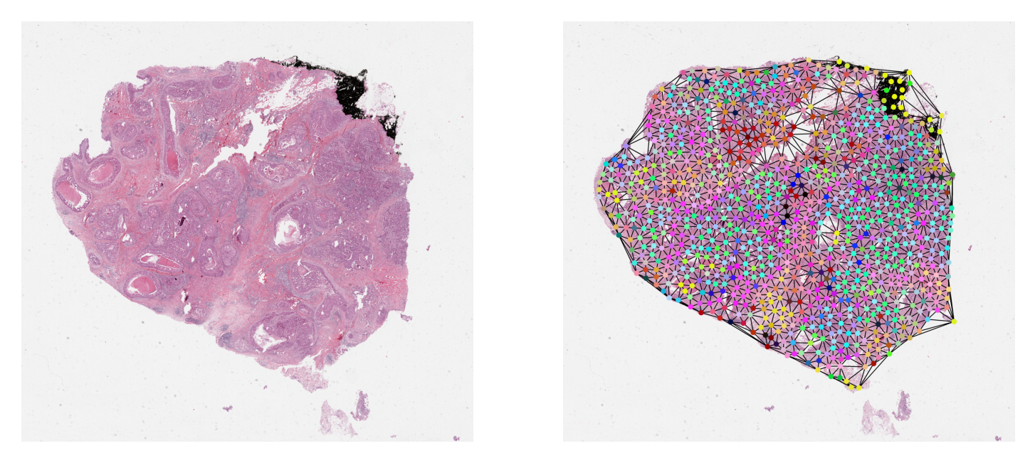
Visualize a Sample Graph

It is always a good practice to visually validate data or any results. Here, we plot one sample graph upon its WSI thumbnail. For illustration purpose, by default we download and plot a sample WSI and its previously generated graph. In order to plot your own WSI or a graph, obtained by running the graph construction code above, you need to comment and uncomment some specific cells below. For more instruction, please read the first comment within each cell.

Aside from that, most of the time the nodes within the graph will be at different resolutions from the resolution at which we want to visualize them. Hence, before plotting, we scale their coordinates to the target resolution. We provide NODE_RESOLUTION and PLOT_RESOLUTION variables respectively as the resolution of the node and the resolution at which to plot the graph.

# By default, we download then visualize a sample WSI and its graph
DOWNLOAD_DIR = "local/dump/"
wsi_path = f"{DOWNLOAD_DIR}/sample.svs"
graph_path = f"{DOWNLOAD_DIR}/graph.json"
mkdir(DOWNLOAD_DIR)

# Downloading sample image tile
URL_HOME = "https://tiatoolbox.dcs.warwick.ac.uk/models/slide_graph/cell-composition"
download_data(
    f"{URL_HOME}/TCGA-C8-A278-01Z-00-DX1.188B3FE0-7B20-401A-A6B7-8F1798018162.svs",
    wsi_path,
)
download_data(
    f"{URL_HOME}/TCGA-C8-A278-01Z-00-DX1.188B3FE0-7B20-401A-A6B7-8F1798018162.json",
    graph_path,
)

Download from https://tiatoolbox.dcs.warwick.ac.uk/models/slide_graph/cell-composition/TCGA-C8-A278-01Z-00-DX1.188B3FE0-7B20-401A-A6B7-8F1798018162.svs
Save to local/dump//sample.svs
Download from https://tiatoolbox.dcs.warwick.ac.uk/models/slide_graph/cell-composition/TCGA-C8-A278-01Z-00-DX1.188B3FE0-7B20-401A-A6B7-8F1798018162.json
Save to local/dump//graph.json

# Uncomment to run later cells to visualize the first WSI within the dataset

# Uncomment and set these variables to run the next cell,
# either separately or with customized parameters
# wsi_path = 'PATH

NODE_SIZE = 24
NODE_RESOLUTION = {"resolution": 0.25, "units": "mpp"}
PLOT_RESOLUTION = {"resolution": 4.0, "units": "mpp"}

graph_dict = load_json(graph_path)
graph_dict = {k: np.array(v) for k, v in graph_dict.items()}
graph = Data(**graph_dict)

# deriving node colors via projecting n-d features down to 3-d
graph.x = StandardScaler().fit_transform(graph.x)
# .c for node colors
node_colors = PCA(n_components=3).fit_transform(graph.x)[:, [1, 0, 2]]
for channel in range(node_colors.shape[-1]):
    node_colors[:, channel] = 1 - equalize_hist(node_colors[:, channel]) ** 2
node_colors = (node_colors * 255).astype(np.uint8)

reader = WSIReader.open(wsi_path)
thumb = reader.slide_thumbnail(4.0, "mpp")

node_resolution = reader.slide_dimensions(**NODE_RESOLUTION)
plot_resolution = reader.slide_dimensions(**PLOT_RESOLUTION)
fx = np.array(node_resolution) / np.array(plot_resolution)

node_coordinates = np.array(graph.coordinates) / fx
edges = graph.edge_index.T

thumb = reader.slide_thumbnail(**PLOT_RESOLUTION)
thumb_overlaid = plot_graph(
    thumb.copy(),
    node_coordinates,
    edges,
    node_colors=node_colors,
    node_size=NODE_SIZE,
)

plt.subplot(1, 2, 1)
plt.imshow(thumb)
plt.axis("off")
plt.subplot(1, 2, 2)
plt.imshow(thumb_overlaid)
plt.axis("off")
plt.show()

The Graph Neural Network

The Dataset Loader

At the time of writing this, graph datasets were not yet supported by TIAToolbox. We therefore defined here their loading and IO conversion. The goal of this dataset class is to support loading the input concurrently, and separately from the running GPU process. The class performs data conversion and other preprocessing if necessary. The preproc argument below is available to specify the function that normalizes node features.

class SlideGraphDataset(Dataset):
    """Handling loading graph data from disk.

    Args:
        info_list (list): In case of `train` or `valid` is in `mode`,
            this is expected to be a list of `[uid, label]` . Otherwise,
            it is a list of `uid`. Here, `uid` is used to construct
            `f"{GRAPH_DIR}/{wsi_code}.json"` which is a path points to
            a `.json` file containing the graph structure. By `label`, we mean
            the label of the graph. The format within the `.json` file comes
            from `tiatoolbox.tools.graph`.
        mode (str): This denotes which data mode the `info_list` is in.
        preproc (callable): The prerocessing function for each node
            within the graph.

    """

    def __init__(
        self: Dataset,
        info_list: list,
        mode: str = "train",
        preproc: Callable | None = None,
    ) -> None:
        """Initialize SlideGraphDataset."""
        self.info_list = info_list
        self.mode = mode
        self.preproc = preproc

    def __getitem__(self: Dataset, idx: int) -> Dataset:
        """Get an element from SlideGraphDataset."""
        info = self.info_list[idx]
        if any(v in self.mode for v in ["train", "valid"]):
            wsi_code, label = info
            # torch.Tensor will create 1-d vector not scalar
            label = torch.tensor(label)
        else:
            wsi_code = info

        with (GRAPH_DIR / str(wsi_code) + ".json").open() as fptr:
            graph_dict = json.load(fptr)
        graph_dict = {k: np.array(v) for k, v in graph_dict.items()}

        if self.preproc is not None:
            graph_dict["x"] = self.preproc(graph_dict["x"])

        graph_dict = {k: torch.tensor(v) for k, v in graph_dict.items()}
        graph = Data(**graph_dict)

        if any(v in self.mode for v in ["train", "valid"]):
            return {"graph": graph, "label": label}
        return {"graph": graph}

    def __len__(self: Dataset) -> int:
        """Length of SlideGraphDataset."""
        return len(self.info_list)

Entire Dataset Feature Normalization

We define the feature normalizer, following the approach used for the stain normalizer. Since this normalization is derived from the entire dataset population, we first load all the node features from all the graphs within our dataset in order to train the normalizer.

To avoid redundancy, we can skip this training step and use an existing normalizer by setting CACHE_PATH to a valid path. By default, the normalizer is trained and saved to SCALER_PATH.

CACHE_PATH = None
SCALER_PATH = f"{ROOT_OUTPUT_DIR}/node_scaler.dat"

# Uncomment and set these variables to run next cell either
# seperately or with customized parameters
# GRAPH_DIR = 'PATH

if CACHE_PATH and CACHE_PATH.exists():
    SCALER_PATH = CACHE_PATH  # assignment for follow up loading
    node_scaler = joblib.load(SCALER_PATH)
else:
    # ! we need a better way of doing this, will have OOM problem
    loader = SlideGraphDataset(wsi_names, mode="infer")
    loader = DataLoader(
        loader,
        num_workers=8,
        batch_size=1,
        shuffle=False,
        drop_last=False,
    )
    node_features = [v["graph"].x.numpy() for idx, v in enumerate(tqdm(loader))]
    node_features = np.concatenate(node_features, axis=0)
    node_scaler = StandardScaler(copy=False)
    node_scaler.fit(node_features)
    joblib.dump(node_scaler, SCALER_PATH)


# we must define the function after training/loading
def nodes_preproc_func(node_features: np.ndarray) -> np.ndarray:
    """Pre-processing function for nodes."""
    return node_scaler.transform(node_features)

100%|██████████| 29/29 [00:00<00:00, 67.27it/s]

GNN Architecture Definition

class SlideGraphArch(nn.Module):
    """Define SlideGraph architecture."""

    def __init__(
        self: nn.Module,
        dim_features: int,
        dim_target: int,
        layers: list[int, int] | None = None,
        pooling: str = "max",
        dropout: float = 0.0,
        conv: str = "GINConv",
        *,
        gembed: bool = False,
        **kwargs: dict,
    ) -> None:
        """Initialize SlideGraphArch."""
        super().__init__()
        if layers is None:
            layers = [6, 6]
        self.dropout = dropout
        self.embeddings_dim = layers
        self.num_layers = len(self.embeddings_dim)
        self.nns = []
        self.convs = []
        self.linears = []
        self.pooling = {
            "max": global_max_pool,
            "mean": global_mean_pool,
            "add": global_add_pool,
        }[pooling]
        # If True then learn a graph embedding for final classification
        # (classify pooled node features), otherwise pool node decision scores.
        self.gembed = gembed

        conv_dict = {"GINConv": [GINConv, 1], "EdgeConv": [EdgeConv, 2]}
        if conv not in conv_dict:
            msg = f'Not support `conv="{conv}".'
            raise ValueError(msg)

        def create_linear(in_dims: int, out_dims: int) -> Linear:
            return nn.Sequential(
                Linear(in_dims, out_dims),
                BatchNorm1d(out_dims),
                ReLU(),
            )

        input_emb_dim = dim_features
        out_emb_dim = self.embeddings_dim[0]
        self.first_h = create_linear(input_emb_dim, out_emb_dim)
        self.linears.append(Linear(out_emb_dim, dim_target))

        input_emb_dim = out_emb_dim
        for out_emb_dim in self.embeddings_dim[1:]:
            conv_class, alpha = conv_dict[conv]
            subnet = create_linear(alpha * input_emb_dim, out_emb_dim)
            # ! this variable should be removed after training integrity checking
            self.nns.append(subnet)  # <--| as it already within ConvClass
            self.convs.append(conv_class(self.nns[-1], **kwargs))
            self.linears.append(Linear(out_emb_dim, dim_target))
            input_emb_dim = out_emb_dim

        self.nns = torch.nn.ModuleList(self.nns)
        self.convs = torch.nn.ModuleList(self.convs)
        # Has got one more for initial input, what does this mean
        self.linears = torch.nn.ModuleList(self.linears)

        # Auxilary holder for external model, these are saved separately from torch.save
        # as they can be sklearn model etc.
        self.aux_model = {}

    def save(self: nn.Module, path: str | Path, aux_path: str | Path) -> None:
        """Save torch model."""
        state_dict = self.state_dict()
        torch.save(state_dict, path)
        joblib.dump(self.aux_model, aux_path)

    def load(self: nn.Module, path: str | Path, aux_path: str | Path) -> None:
        """Load torch model."""
        state_dict = torch.load(path)
        self.load_state_dict(state_dict)
        self.aux_model = joblib.load(aux_path)

    def forward(self: nn.Module, data: np.ndarray | torch.Tensor) -> tuple:
        """Torch model forward function."""
        feature, edge_index, batch = data.x, data.edge_index, data.batch

        wsi_prediction = 0
        pooling = self.pooling
        node_prediction = 0

        feature = self.first_h(feature)
        for layer in range(self.num_layers):
            if layer == 0:
                node_prediction_sub = self.linears[layer](feature)
                node_prediction += node_prediction_sub
                node_pooled = pooling(node_prediction_sub, batch)
                wsi_prediction_sub = F.dropout(
                    node_pooled,
                    p=self.dropout,
                    training=self.training,
                )
                wsi_prediction += wsi_prediction_sub
            else:
                feature = self.convs[layer - 1](feature, edge_index)
                if not self.gembed:
                    node_prediction_sub = self.linears[layer](feature)
                    node_prediction += node_prediction_sub
                    node_pooled = pooling(node_prediction_sub, batch)
                    wsi_prediction_sub = F.dropout(
                        node_pooled,
                        p=self.dropout,
                        training=self.training,
                    )
                else:
                    node_pooled = pooling(feature, batch)
                    node_prediction_sub = self.linears[layer](node_pooled)
                    wsi_prediction_sub = F.dropout(
                        node_prediction_sub,
                        p=self.dropout,
                        training=self.training,
                    )
                wsi_prediction += wsi_prediction_sub
        return wsi_prediction, node_prediction

    # Run one single step
    @staticmethod
    def train_batch(
        model: nn.Module,
        batch_data: np.ndarray | torch.Tensor,
        optimizer: torch.optim.Optimizer,
        device: str,
    ) -> list:
        """Helper function for model training."""
        wsi_graphs = batch_data["graph"].to(device)
        wsi_labels = batch_data["label"].to(device)
        model = model.to(device)

        # Data type conversion
        wsi_graphs.x = wsi_graphs.x.type(torch.float32)

        # Not an RNN so does not accumulate
        model.train()
        optimizer.zero_grad()

        wsi_output, _ = model(wsi_graphs)

        # Both are expected to be Nx1
        wsi_labels_ = wsi_labels[:, None]
        wsi_labels_ = wsi_labels_ - wsi_labels_.T
        wsi_output_ = wsi_output - wsi_output.T
        diff = wsi_output_[wsi_labels_ > 0]
        loss = torch.mean(F.relu(1.0 - diff))
        # Backprop and update
        loss.backward()
        optimizer.step()

        loss = loss.detach().cpu().numpy()
        assert not np.isnan(loss)  # noqa: S101
        wsi_labels = wsi_labels.cpu().numpy()
        return [loss, wsi_output, wsi_labels]

    # Run one inference step
    @staticmethod
    def infer_batch(
        model: nn.Module,
        batch_data: torch.Tensor,
        device: str,
    ) -> list:
        """Model inference."""
        wsi_graphs = batch_data["graph"].to(device)
        model = model.to(device)

        # Data type conversion
        wsi_graphs.x = wsi_graphs.x.type(torch.float32)

        # Inference mode
        model.eval()
        # Do not compute the gradient (not training)
        with torch.inference_mode():
            wsi_output, _ = model(wsi_graphs)

        wsi_output = wsi_output.cpu().numpy()
        # Output should be a single tensor or scalar
        if "label" in batch_data:
            wsi_labels = batch_data["label"]
            wsi_labels = wsi_labels.cpu().numpy()
            return wsi_output, wsi_labels
        return [wsi_output]

To test that our architecture works, at least superficially, we perform a brief inference with some random graph data and print out the output predictions.

# Uncomment and set these variables to run next cell either
# seperately or with customized parameters

dummy_ds = SlideGraphDataset(wsi_names, mode="infer")
loader = DataLoader(
    dummy_ds,
    num_workers=0,
    batch_size=8,
    shuffle=False,
)
iterator = iter(loader)
batch_data = iterator.__next__()

# Data type conversion
wsi_graphs = batch_data["graph"]
wsi_graphs.x = wsi_graphs.x.type(torch.float32)

# Define model object
arch_kwargs = {
    "dim_features": NUM_NODE_FEATURES,
    "dim_target": 1,
    "layers": [16, 16, 8],
    "dropout": 0.5,
    "pooling": "mean",
    "conv": "EdgeConv",
    "aggr": "max",
}
model = SlideGraphArch(**arch_kwargs)

# Inference section
model.eval()
with torch.inference_mode():
    output, _ = model(wsi_graphs)
    output = output.cpu().numpy()
logger.info(
    "Output [%f, %f, %f, %f, %f, %f, %f, %f]",
    output[0][0],
    output[0][1],
    output[0][2],
    output[0][3],
    output[0][4],
    output[0][5],
    output[0][6],
    output[0][7],
)

[[-5.274482 ]
 [-5.2743864]
 [-5.2757716]
 [-5.27656  ]
 [-5.272782 ]
 [-5.2744055]
 [-5.274012 ]
 [-5.27648  ]]

Notice that the output values do not lie in the interval [0,1]. Later we will turn the above values into probabilities using Platt Scaling. The scaler will be defined and trained during the training process defined below. After training is complete, the scaler can be accessed with:

model = SlideGraphArch(**arch_kwargs)
model.aux_model  # will hold the trained Platt Scaler

Batch Sampler

Now that we have ensured that the model can run, let’s take a step back and look at the model definition again, in preparation for training and inference handling.

The infer_batch is straightforward here: it handles inferencing of the input batch data and organizes the output content. Likewise, train_batch defines training, such as calculating the loss and so on. The loss defined here is not straightforward or standardized like cross-entropy. There is a pitfall lurking in the above code that could crash the training. Consider the lines:

wsi_labels_ = wsi_labels[:, None]
wsi_labels_ = wsi_labels_ - wsi_labels_.T
wsi_output_ = wsi_output - wsi_output.T
diff = wsi_output_[wsi_labels_ > 0]
loss = torch.mean(F.relu(1.0 - diff))

Specifically, we need to take care of diff = wsi_output_[wsi_labels_ > 0] where we want to calculate the loss using only positive samples. When a batch contains no positive samples at all, especially for a skewed dataset, there will no samples to calculate the loss and we will have NaN loss. To resolve this, we define a sampler specifically for the training process, such that its resulting batch always contains positive samples.

class StratifiedSampler(Sampler):
    """Sampling the dataset such that the batch contains stratified samples.

    Args:
        labels (list): List of labels, must be in the same ordering as input
            samples provided to the `SlideGraphDataset` object.
        batch_size (int): Size of the batch.

    Returns:
        List of indices to query from the `SlideGraphDataset` object.

    """

    def __init__(self: Sampler, labels: list, batch_size: int = 10) -> None:
        """Initialize StratifiedSampler."""
        self.batch_size = batch_size
        self.num_splits = int(len(labels) / self.batch_size)
        self.labels = labels
        self.num_steps = self.num_splits

    def _sampling(self: Sampler) -> list:
        """Do we want to control randomness here."""
        skf = StratifiedKFold(n_splits=self.num_splits, shuffle=True)
        indices = np.arange(len(self.labels))  # idx holder
        # return array of arrays of indices in each batch
        return [tidx for _, tidx in skf.split(indices, self.labels)]

    def __iter__(self: Sampler) -> Iterator:
        """Define Iterator."""
        return iter(self._sampling())

    def __len__(self: Sampler) -> int:
        """The length of the sampler.

        This value actually corresponds to the number of steps to query
        sampled batch indices. Thus, to maintain epoch and steps hierarchy,
        this should be equal to the number of expected steps as in usual
        sampling: `steps=dataset_size / batch_size`.

        """
        return self.num_steps

The Training Loop

Training and running a neural network at the current time involves plugging several parts together so that they work in tandem. In simplified terms, training consists of the following steps:

1. Define a network object (torch.nn.module) for a particular architecture.

2. Define a loader object to handle loading data concurrently.

3. Define an optimizer(s) and scheduler to update the network weights.

4. Define callback functions for several stages (starting of epoch, end of step, etc.) to aggregate results, save the models, refresh data, and much more.

For inference, #3 is not necessary.

At the moment, the wiring of these operations is handled mostly by various engine classes within the toolbox. However, they focus mostly on the inference portion. For the SlideGraph case and this notebook, we also require the engine to handle the training portion. Hence, we define below a very simplified version of what an engine usually does for both training and inference.

Helper Functions & Classes

The function create_pbar simplifies the process of creating a progress bar for tracking the running loop. We also define a class to calculate the exponential moving average (EMA) of the training loss for each step.

def create_pbar(subset_name: str, num_steps: int) -> tqdm:
    """Create a nice progress bar."""
    pbar_format = (
        "Processing: |{bar}| {n_fmt}/{total_fmt}[{elapsed}<{remaining},{rate_fmt}]"
    )
    pbar = tqdm(total=num_steps, leave=True, bar_format=pbar_format, ascii=True)
    if subset_name == "train":
        pbar_format += "step={postfix[1][step]:0.5f}|EMA={postfix[1][EMA]:0.5f}"
        # * Changing print char may break the bar so avoid it
        pbar = tqdm(
            total=num_steps,
            leave=True,
            initial=0,
            bar_format=pbar_format,
            ascii=True,
            postfix=["", {"step": float("NaN"), "EMA": float("NaN")}],
        )
    return pbar


class ScalarMovingAverage:
    """Class to calculate running average."""

    def __init__(self: ScalarMovingAverage, alpha: float = 0.95) -> None:
        """Initialize ScalarMovingAverage."""
        super().__init__()
        self.alpha = alpha
        self.tracking_dict = {}

    def __call__(self: ScalarMovingAverage, step_output: dict) -> None:
        """ScalarMovingAverage instances behave and can be called like a function."""
        for key, current_value in step_output.items():
            if key in self.tracking_dict:
                old_ema_value = self.tracking_dict[key]
                # Calculate the exponential moving average
                new_ema_value = (
                    old_ema_value * self.alpha + (1.0 - self.alpha) * current_value
                )
                self.tracking_dict[key] = new_ema_value
            else:  # Init for variable which appear for the first time
                new_ema_value = current_value
                self.tracking_dict[key] = new_ema_value

Defining The Loop

Finally, we define the function to manage the running loop, or the simplified engine so to speak. The running loop contains of several important events that require special definition and handling of the dataset, the model, etc.

• EPOCH_START: The start of each epoch. Depending on the task, it may be necessary to clean up and refresh the data accumulated over the previous epoch (such as clearing previous validation results).

• STEP_START: The start of each step. The loader is asked for data. The data is passed on and training or model inference step is triggered.

• STEP_STOP: The end of each step. The loss is computed, console output is logged, and the training or inference results are collated.

• EPOCH_COMPLETE: The end of each epoch. This often involves saving the model, or in our case, starting the training of the Platt Scaler.

Often, each of these events has its own set of callbacks that will be invoked. Furthermore, these callbacks may also vary with dataset or running mode (such as metric calculations, saving mode, etc.). As this is a simplified version, we include all handling of these within run_once. In practice, they are usually factored out into a set of classes and hooks.

The run_once function is provided with a dictionary of datasets. Within this dictionary, train is the dataset used for training which includes the sampler that ensures a positive sample in each batch. Additionally, *infer-valid* and *infer-train* are the datasets used for validation of the model and training of the Platt scaling respectively. These two datasets do not make use of the sampler ensuring a positive sample in each batch. Any other dataset in the dictionary which matches the pattern *infer* is assumed to be used for testing.

def run_once(  # noqa: C901, PLR0912, PLR0915
    dataset_dict: dict,
    num_epochs: int,
    save_dir: str | Path,
    pretrained: str | None = None,
    loader_kwargs: dict | None = None,
    arch_kwargs: dict | None = None,
    optim_kwargs: dict | None = None,
    device: str = "cuda",
) -> list:
    """Running the inference or training loop once.

    The actual running mode is defined via the code name of the dataset
    within `dataset_dict`. Here, `train` is specifically preserved for
    the dataset used for training. `.*infer-valid.*` and `.*infer-train*`
    are reserved for datasets containing the corresponding labels.
    Otherwise, the dataset is assumed to be for the inference run.

    """
    if loader_kwargs is None:
        loader_kwargs = {}

    if arch_kwargs is None:
        arch_kwargs = {}

    if optim_kwargs is None:
        optim_kwargs = {}

    model = SlideGraphArch(**arch_kwargs)
    if pretrained is not None:
        model.load(*pretrained)
    model = model.to("cuda")
    optimizer = torch.optim.Adam(model.parameters(), **optim_kwargs)

    # Create the graph dataset holder for each subset info then
    # pipe them through torch/torch geometric specific loader
    # for loading in multi-thread.
    loader_dict = {}
    for subset_name, subset in dataset_dict.items():
        _loader_kwargs = copy.deepcopy(loader_kwargs)
        batch_sampler = None
        if subset_name == "train":
            _loader_kwargs = {}
            batch_sampler = StratifiedSampler(
                labels=[v[1] for v in subset],
                batch_size=loader_kwargs["batch_size"],
            )

        ds = SlideGraphDataset(subset, mode=subset_name, preproc=nodes_preproc_func)
        loader_dict[subset_name] = DataLoader(
            ds,
            batch_sampler=batch_sampler,
            drop_last=subset_name == "train" and batch_sampler is None,
            shuffle=subset_name == "train" and batch_sampler is None,
            **_loader_kwargs,
        )

    for epoch in range(num_epochs):
        logger.info("EPOCH: %03d", epoch)
        for loader_name, loader in loader_dict.items():
            # * EPOCH START
            step_output = []
            ema = ScalarMovingAverage()
            pbar = create_pbar(loader_name, len(loader))
            for _step, batch_data in enumerate(loader):
                # * STEP COMPLETE CALLBACKS
                if loader_name == "train":
                    output = model.train_batch(model, batch_data, device, optimizer)
                    # check the output for agreement
                    ema({"loss": output[0]})
                    pbar.postfix[1]["step"] = output[0]
                    pbar.postfix[1]["EMA"] = ema.tracking_dict["loss"]
                else:
                    output = model.infer_batch(model, batch_data, device)

                    batch_size = batch_data["graph"].num_graphs
                    # Iterate over output head and retrieve
                    # each as N x item, each item may be of
                    # arbitrary dimensions
                    output = [np.split(v, batch_size, axis=0) for v in output]
                    # pairing such that it will be
                    # N batch size x H head list
                    output = list(zip(*output))
                    step_output.extend(output)
                pbar.update()
            pbar.close()

            # * EPOCH COMPLETE

            # Callbacks to process output
            logging_dict = {}
            if loader_name == "train":
                for val_name, val in ema.tracking_dict.items():
                    logging_dict[f"train-EMA-{val_name}"] = val
            elif "infer" in loader_name and any(
                v in loader_name for v in ["train", "valid"]
            ):
                # Expand the list of N dataset size x H heads
                # back to a list of H Head each with N samples.
                output = list(zip(*step_output))
                logit, true = output
                logit = np.squeeze(np.array(logit))
                true = np.squeeze(np.array(true))

                if "train" in loader_name:
                    scaler = PlattScaling()
                    scaler.fit(np.array(logit, ndmin=2).T, true)
                    model.aux_model["scaler"] = scaler
                scaler = model.aux_model["scaler"]
                prob = scaler.predict_proba(np.array(logit, ndmin=2).T)[:, 0]

                val = auroc_scorer(true, prob)
                logging_dict[f"{loader_name}-auroc"] = val
                val = auprc_scorer(true, prob)
                logging_dict[f"{loader_name}-auprc"] = val

                logging_dict[f"{loader_name}-raw-logit"] = logit
                logging_dict[f"{loader_name}-raw-true"] = true

            # Callbacks for logging and saving
            for val_name, val in logging_dict.items():
                if "raw" not in val_name:
                    logging.info("%s: %d:", val_name, val)
            if "train" not in loader_dict:
                continue

            # Track the statistics
            new_stats = {}
            if (save_dir / "stats.json").exists():
                old_stats = load_json(f"{save_dir}/stats.json")
                # Save a backup first
                save_as_json(old_stats, f"{save_dir}/stats.old.json", exist_ok=False)
                new_stats = copy.deepcopy(old_stats)
                new_stats = {int(k): v for k, v in new_stats.items()}

            old_epoch_stats = {}
            if epoch in new_stats:
                old_epoch_stats = new_stats[epoch]
            old_epoch_stats.update(logging_dict)
            new_stats[epoch] = old_epoch_stats
            save_as_json(new_stats, f"{save_dir}/stats.json", exist_ok=False)

            # Save the pytorch model
            model.save(
                f"{save_dir}/epoch={epoch:03d}.weights.pth",
                f"{save_dir}/epoch={epoch:03d}.aux.dat",
            )
    return step_output

logging.basicConfig(
    level=logging.INFO,
)


def reset_logging(save_path: str | Path) -> None:
    """Reset logger handler."""
    log_formatter = logging.Formatter(
        "|%(asctime)s.%(msecs)03d| [%(levelname)s] %(message)s",
        datefmt="%Y-%m-%d|%H:%M:%S",
    )
    log = logging.getLogger()  # Root logger
    for hdlr in log.handlers[:]:  # Remove all old handlers
        log.removeHandler(hdlr)
    new_hdlr_list = [
        logging.FileHandler(f"{save_path}/debug.log"),
        logging.StreamHandler(),
    ]
    for hdlr in new_hdlr_list:
        hdlr.setFormatter(log_formatter)
        log.addHandler(hdlr)

Training

With the engine above, we can now start our training loop with a set of parameters:

• MODEL_DIR: the location where we save the model weights and associated information every epoch. Under it, we have

  • epoch=[X].weights.pth: the graph neural network weights after the X-th training epoch.

  • epoch=[X].weights.aux.dat: the associated sklearn model trained for the X-th epoch. In our case, it contains the Platt Scaling.

  • stats.json: the file contains accumulated statistic of the entire training run for the X-th epoch.

  • stats.old.json: the backup file of stats.json of the previous epoch.

• NUM_EPOCHS: the number of epoch for training.

To avoid accidentally over-writing training results, we will skip training if MODEL_DIR already exists.

# Default parameters
NUM_EPOCHS = 100
NUM_NODE_FEATURES = 4
SCALER_PATH = f"{ROOT_OUTPUT_DIR}/node_scaler.dat"
MODEL_DIR = f"{ROOT_OUTPUT_DIR}/model/"

# Uncomment and set these variables to run next cell either
# seperately or with customized parameters

splits = joblib.load(SPLIT_PATH)
node_scaler = joblib.load(SCALER_PATH)
loader_kwargs = {
    "num_workers": 8,
    "batch_size": 16,
}
arch_kwargs = {
    "dim_features": NUM_NODE_FEATURES,
    "dim_target": 1,
    "layers": [16, 16, 8],
    "dropout": 0.5,
    "pooling": "mean",
    "conv": "EdgeConv",
    "aggr": "max",
}
optim_kwargs = {
    "lr": 1.0e-3,
    "weight_decay": 1.0e-4,
}


if not MODEL_DIR.exists():
    for split_idx, split in enumerate(splits):
        new_split = {
            "train": split["train"],
            "infer-train": split["train"],
            "infer-valid-A": split["valid"],
            "infer-valid-B": split["test"],
        }
        split_save_dir = f"{MODEL_DIR}/{split_idx:02d}/"
        rm_n_mkdir(split_save_dir)
        reset_logging(split_save_dir)
        run_once(
            new_split,
            NUM_EPOCHS,
            save_dir=split_save_dir,
            arch_kwargs=arch_kwargs,
            loader_kwargs=loader_kwargs,
            optim_kwargs=optim_kwargs,
        )

Inference

Model Selections

According to our engine running loop defined above, we will have the following metrics saved for each epoch:

• “infer-train-auroc”

• “infer-train-auprc”

• “infer-valid-auroc”

• “infer-valid-auprc”

With these metrics, we can pick the most promising model weights for inference on an independent dataset. We encapsulate this selection within the select_checkpoints function.

Note: For the metrics we defined here (auroc, auprc), a larger value is better. If you want to add your own metrics, remember to change the comparison operators within select_checkpoints function accordingly.

def select_checkpoints(
    stat_file_path: str,
    top_k: int = 2,
    metric: str = "infer-valid-auprc",
    epoch_range: tuple[int] | None = None,
) -> tuple[list, list]:
    """Select checkpoints basing on training statistics.

    Args:
        stat_file_path (str): Path pointing to the .json
            which contains the statistics.
        top_k (int): Number of top checkpoints to be selected.
        metric (str): The metric name saved within .json to perform
            selection.
        epoch_range (list): The range of epochs for checking, denoted
            as [start, end] . Epoch x that is `start <= x <= end` is
            kept for further selection.

    Returns:
        paths (list): List of paths or info tuple where each point
            to the correspond check point saving location.
        stats (list): List of corresponding statistics.

    """
    if epoch_range is None:
        epoch_range = [0, 1000]
    stats_dict = load_json(stat_file_path)
    # k is the epoch counter in this case
    stats_dict = {
        k: v
        for k, v in stats_dict.items()
        if int(k) >= epoch_range[0] and int(k) <= epoch_range[1]
    }
    stats = [[int(k), v[metric], v] for k, v in stats_dict.items()]
    # sort epoch ranking from largest to smallest
    stats = sorted(stats, key=lambda v: v[1], reverse=True)
    chkpt_stats_list = stats[:top_k]  # select top_k

    model_dir = Path(stat_file_path).parent
    epochs = [v[0] for v in chkpt_stats_list]
    paths = [
        (
            f"{model_dir}/epoch={epoch:03d}.weights.pth",
            f"{model_dir}/epoch={epoch:03d}.aux.dat",
        )
        for epoch in epochs
    ]
    chkpt_stats_list = [[v[0], v[2]] for v in chkpt_stats_list]
    print(paths)  # noqa: T201
    return paths, chkpt_stats_list

Bulk Inference & Ensemble Results

# default parameters
TOP_K = 1
metric_name = "infer-valid-B-auroc"
PRETRAINED_DIR = f"{ROOT_OUTPUT_DIR}/model/"
SCALER_PATH = f"{ROOT_OUTPUT_DIR}/node_scaler.dat"

# Uncomment and set these variables to run the next cell,
# either seperately or with customized parameters

splits = joblib.load(SPLIT_PATH)
node_scaler = joblib.load(SCALER_PATH)
loader_kwargs = {
    "num_workers": 8,
    "batch_size": 16,
}
arch_kwargs = {
    "dim_features": NUM_NODE_FEATURES,
    "dim_target": 1,
    "layers": [16, 16, 8],
    "dropout": 0.5,
    "pooling": "mean",
    "conv": "EdgeConv",
    "aggr": "max",
}

cum_stats = []
for split_idx, split in enumerate(splits):
    new_split = {"infer": [v[0] for v in split["test"]]}

    stat_files = recur_find_ext(f"{PRETRAINED_DIR}/{split_idx:02d}/", [".json"])
    stat_files = [v for v in stat_files if ".old.json" not in v]
    assert len(stat_files) == 1  # noqa: S101
    chkpts, chkpt_stats_list = select_checkpoints(
        stat_files[0],
        top_k=TOP_K,
        metric=metric_name,
    )

    # Perform ensembling by averaging probabilities
    # across checkpoint predictions
    cum_results = []
    for chkpt_info in chkpts:
        chkpt_results = run_once(
            new_split,
            num_epochs=1,
            save_dir=None,
            pretrained=chkpt_info,
            arch_kwargs=arch_kwargs,
            loader_kwargs=loader_kwargs,
        )
        # * re-calibrate logit to probabilities
        model = SlideGraphArch(**arch_kwargs)
        model.load(*chkpt_info)
        scaler = model.aux_model["scaler"]
        chkpt_results = np.array(chkpt_results)
        chkpt_results = np.squeeze(chkpt_results)
        chkpt_results = scaler.transform(chkpt_results)

        cum_results.append(chkpt_results)
    cum_results = np.array(cum_results)
    cum_results = np.squeeze(cum_results)

    prob = cum_results
    if len(cum_results.shape) == 2:  # noqa: PLR2004
        prob = np.mean(cum_results, axis=0)

    # * Calculate split statistics
    true = [v[1] for v in split["test"]]
    true = np.array(true)

    cum_stats.append(
        {"auroc": auroc_scorer(true, prob), "auprc": auprc_scorer(true, prob)},
    )

[('/home/dang/storage_1/workspace/tiatoolbox/local/slidegraph/storage/nima/dump/model/00/epoch=073.weights.pth', '/home/dang/storage_1/workspace/tiatoolbox/local/slidegraph/storage/nima/dump/model/00/epoch=073.aux.dat')]

|2021-11-03|18:19:51.309| [INFO] EPOCH 000
Processing: |##########| 10/10[00:00<00:00,15.10it/s]
|2021-11-03|18:19:52.015| [INFO] EPOCH 000
Processing: |          | 0/10[00:00<?,?it/s]

[('/home/dang/storage_1/workspace/tiatoolbox/local/slidegraph/storage/nima/dump/model/01/epoch=086.weights.pth', '/home/dang/storage_1/workspace/tiatoolbox/local/slidegraph/storage/nima/dump/model/01/epoch=086.aux.dat')]

Processing: |##########| 10/10[00:00<00:00,15.42it/s]
|2021-11-03|18:19:52.706| [INFO] EPOCH 000
Processing: |          | 0/10[00:00<?,?it/s]

[('/home/dang/storage_1/workspace/tiatoolbox/local/slidegraph/storage/nima/dump/model/02/epoch=003.weights.pth', '/home/dang/storage_1/workspace/tiatoolbox/local/slidegraph/storage/nima/dump/model/02/epoch=003.aux.dat')]

Processing: |##########| 10/10[00:00<00:00,14.10it/s]
|2021-11-03|18:19:53.472| [INFO] EPOCH 000
Processing: |          | 0/10[00:00<?,?it/s]

[('/home/dang/storage_1/workspace/tiatoolbox/local/slidegraph/storage/nima/dump/model/03/epoch=009.weights.pth', '/home/dang/storage_1/workspace/tiatoolbox/local/slidegraph/storage/nima/dump/model/03/epoch=009.aux.dat')]

Processing: |##########| 10/10[00:00<00:00,15.27it/s]
|2021-11-03|18:19:54.162| [INFO] EPOCH 000
Processing: |          | 0/10[00:00<?,?it/s]

[('/home/dang/storage_1/workspace/tiatoolbox/local/slidegraph/storage/nima/dump/model/04/epoch=085.weights.pth', '/home/dang/storage_1/workspace/tiatoolbox/local/slidegraph/storage/nima/dump/model/04/epoch=085.aux.dat')]

Processing: |##########| 10/10[00:00<00:00,14.80it/s]

Now we print out the results.

stat_df = pd.DataFrame(cum_stats)
for metric in stat_df.columns:
    vals = stat_df[metric]
    mu = np.mean(vals)
    va = np.std(vals)
    logger.info(" %s: %0.4f±%0.4f", metric, mu, va)

auroc: 0.7380±0.0433
auprc: 0.3541±0.0747

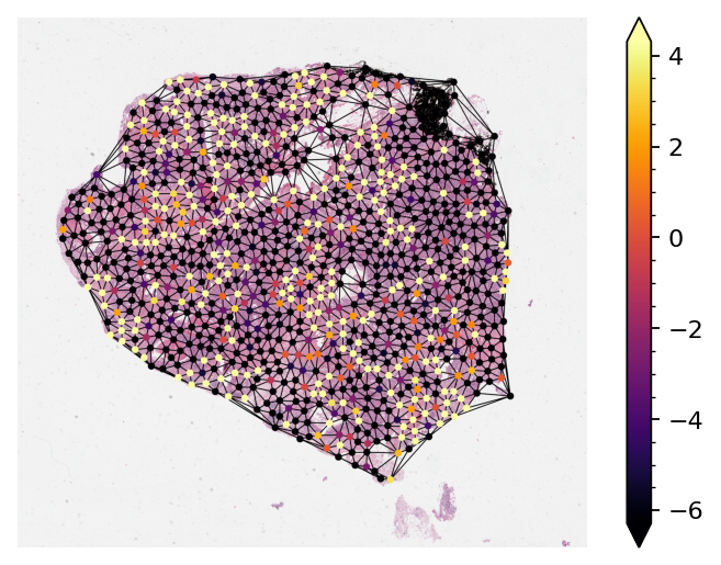
Visualizing Node Activation of the Graph Neural Network

Visualizing the activations of each node within the graph is sometimes necessary to either debug or verify the predictions of the graph neural network. Here, we demonstrate

1. Loading a pretrained model and running inference on one single sample graph.

2. Retrieving the node activations and plot them on the original WSI.

By default, notice that node activations are output when running the mode.forward(input) (Or simply model(input) in pytorch).

By default, we download the pretrained model as well as samples from the tiatoolbox server to DOWNLOAD_DIR. However, if you want to use your own set of input, you can comment out the next cell and provide your own data.

# ! If you want to run your own set of input, comment out this cell
# ! and uncomment the next cell
DOWNLOAD_DIR = "local/dump/"
WSI_PATH = f"{DOWNLOAD_DIR}/sample.svs"
GRAPH_PATH = f"{DOWNLOAD_DIR}/graph.json"
SCALER_PATH = f"{DOWNLOAD_DIR}/node_scaler.dat"
MODEL_WEIGHTS_PATH = f"{DOWNLOAD_DIR}/model.weigths.pth"
MODEL_AUX_PATH = f"{DOWNLOAD_DIR}/model.aux.dat"
mkdir(DOWNLOAD_DIR)

# Downloading sample image tile
URL_HOME = "https://tiatoolbox.dcs.warwick.ac.uk/models/slide_graph/cell-composition"
download_data(
    f"{URL_HOME}/TCGA-C8-A278-01Z-00-DX1.188B3FE0-7B20-401A-A6B7-8F1798018162.svs",
    WSI_PATH,
)
download_data(
    f"{URL_HOME}/TCGA-C8-A278-01Z-00-DX1.188B3FE0-7B20-401A-A6B7-8F1798018162.json",
    GRAPH_PATH,
)
download_data(f"{URL_HOME}/node_scaler.dat", SCALER_PATH)
download_data(f"{URL_HOME}/model.aux.dat", MODEL_AUX_PATH)
download_data(f"{URL_HOME}/model.weights.pth", MODEL_WEIGHTS_PATH)

Download from https://tiatoolbox.dcs.warwick.ac.uk/models/slide_graph/cell-composition/TCGA-C8-A278-01Z-00-DX1.188B3FE0-7B20-401A-A6B7-8F1798018162.svs
Save to local/dump//sample.svs
Download from https://tiatoolbox.dcs.warwick.ac.uk/models/slide_graph/cell-composition/TCGA-C8-A278-01Z-00-DX1.188B3FE0-7B20-401A-A6B7-8F1798018162.json
Save to local/dump//graph.json
Download from https://tiatoolbox.dcs.warwick.ac.uk/models/slide_graph/cell-composition/node_scaler.dat
Save to local/dump//node_scaler.dat
Download from https://tiatoolbox.dcs.warwick.ac.uk/models/slide_graph/cell-composition/model.aux.dat
Save to local/dump//model.aux.dat
Download from https://tiatoolbox.dcs.warwick.ac.uk/models/slide_graph/cell-composition/model.weights.pth
Save to local/dump//model.weigths.pth

# If you want to run your own set of input,
# uncomment these lines and then set variables to run next cell

Most of the time the nodes within the graph will be at different resolutions from the resolution at which we want to visualize them. Before plotting, we scale their coordinates to the target resolution. We provide NODE_RESOLUTION and PLOT_RESOLUTION variables respectively as the resolution of the node and the resolution at which to plot the graph.

NODE_SIZE = 25
NUM_NODE_FEATURES = 4
NODE_RESOLUTION = {"resolution": 0.25, "units": "mpp"}
PLOT_RESOLUTION = {"resolution": 4.0, "units": "mpp"}

node_scaler = joblib.load(SCALER_PATH)
loader_kwargs = {
    "num_workers": 8,
    "batch_size": 16,
}
arch_kwargs = {
    "dim_features": NUM_NODE_FEATURES,
    "dim_target": 1,
    "layers": [16, 16, 8],
    "dropout": 0.5,
    "pooling": "mean",
    "conv": "EdgeConv",
    "aggr": "max",
}


with GRAPH_PATH.open() as fptr:
    graph_dict = json.load(fptr)
graph_dict = {k: np.array(v) for k, v in graph_dict.items()}
graph_dict["x"] = node_scaler.transform(graph_dict["x"])
graph_dict = {k: torch.tensor(v) for k, v in graph_dict.items()}
graph = Data(**graph_dict)
batch = Batch.from_data_list([graph])

model = SlideGraphArch(**arch_kwargs)
model.load(MODEL_WEIGHTS_PATH, MODEL_AUX_PATH)
model = model.to("cuda")

# Data type conversion
batch = batch.to("cuda")
batch.x = batch.x.type(torch.float32)
predictions, node_activations = model(batch)
node_activations = node_activations.detach().cpu().numpy()

reader = OpenSlideWSIReader(WSI_PATH)
node_resolution = reader.slide_dimensions(**NODE_RESOLUTION)
plot_resolution = reader.slide_dimensions(**PLOT_RESOLUTION)
fx = np.array(node_resolution) / np.array(plot_resolution)

cmap = plt.get_cmap("inferno")
graph = graph.to("cpu")

node_coordinates = np.array(graph.coordinates) / fx
node_colors = (cmap(np.squeeze(node_activations))[..., :3] * 255).astype(np.uint8)
edges = graph.edge_index.T

thumb = reader.slide_thumbnail(**PLOT_RESOLUTION)
thumb_overlaid = plot_graph(
    thumb.copy(),
    node_coordinates,
    edges,
    node_colors=node_colors,
    node_size=NODE_SIZE,
)

ax = plt.subplot(1, 1, 1)
plt.imshow(thumb_overlaid)
plt.axis("off")
# Add minorticks on the colorbar to make it easy to read the
# values off the colorbar.
fig = plt.gcf()
norm = mpl.colors.Normalize(
    vmin=np.min(node_activations),
    vmax=np.max(node_activations),
)
sm = plt.cm.ScalarMappable(cmap=cmap, norm=norm)
cbar = fig.colorbar(sm, ax=ax, extend="both")
cbar.minorticks_on()
plt.show()