Whole Slide Image Registration

Click to open in: [GitHub][Colab]

About this notebook

This Jupyter notebook can be run on any computer with a standard browser and no prior installation of any programming language is required. It can run remotely over the Internet, free of charge, thanks to Google Colaboratory. To connect with Colab, click on one of the two blue checkboxes above. Check that “colab” appears in the address bar. You can right-click on “Open in Colab” and select “Open in new tab” if the left click does not work for you. Familiarize yourself with the drop-down menus near the top of the window. You can edit the notebook during the session, for example substituting your own image files for the image files used in this demo. Experiment by changing the parameters of functions. It is not possible for an ordinary user to permanently change this version of the notebook on GitHub or Colab, so you cannot inadvertently mess it up. Use the notebook’s File Menu if you wish to save your own (changed) notebook.

To run the notebook on any platform, except for Colab, set up your Python environment, as explained in the README file.

About this demo

In this example, we will show how to use TIAToolbox for registration of a pair of histology images. Registration refers to aligning a pair of images where one of the images is referred to as the fixed image while the other image is referred as the moving image. The moving image is spatially transformed so that it aligns with the fixed image. Registration often serves as an essential pre-processing step for many medical image analysis tasks. Registration of multiple sections in a tissue block is an important pre-requisite task before any cross-slide image analysis.

We perform registration of an image pair using Deep Feature Based Registration (DFBR) [1], followed by non-rigid alignment using SimpleITK. The registration tool in the TIAToolbox also comprises a pre-alignment step, pre-requisite to DFBR. In particular, we will introduce the use of our registration tool wsi_registration.

[1] Awan, Ruqayya, et al. “Deep Feature based Cross-slide Registration.” arXiv preprint arXiv:2202.09971 (2022).

Setting up the environment

TIAToolbox and dependencies installation

You can skip the following cell if 1) you are not using the Colab plaform or 2) you are using Colab and this is not your first run of the notebook in the current runtime session. If you nevertheless run the cell, you may get an error message, but no harm will be done. On Colab the cell installs tiatoolbox, and other prerequisite software. Harmless error messages should be ignored. Outside Colab , the notebook expects tiatoolbox to already be installed. (See the instructions in README.)

%%bash
apt-get -y install libopenjp2-7-dev libopenjp2-tools openslide-tools libpixman-1-dev | tail -n 1
pip install git+https://github.com/TissueImageAnalytics/tiatoolbox.git@develop | tail -n 1
echo "Installation is done."

IMPORTANT: When you run the cell above for the first time, while using Colab, you need to restart the runtime before proceeding further. Click on the box RESTART RUNTIME that appears immediately above this cell, or use the menu Runtime→Restart runtime. This loads the latest versions of prerequisite packages. The notebook can then be managed normally. For example, you can run subsequent cells one by one, or you can click on Runtime→Run all or Runtime→after.

Importing related libraries

We import some standard Python modules, and also the TIAToolbox Python modules for the image registration task, written by the TIA Centre team.

"""Import modules required to run the Jupyter notebook."""

from __future__ import annotations

# Clear logger to use tiatoolbox.logger
import logging

if logging.getLogger().hasHandlers():
    logging.getLogger().handlers.clear()

import shutil
import warnings
from pathlib import Path

import cv2
import matplotlib as mpl
import numpy as np
import requests
from matplotlib import pyplot as plt
from scipy import ndimage
from skimage import color, exposure, measure, morphology

from tiatoolbox import logger
from tiatoolbox.models.engine.semantic_segmentor import SemanticSegmentor
from tiatoolbox.tools.registration.wsi_registration import (
    AffineWSITransformer,
    DFBRegister,
    apply_bspline_transform,
    estimate_bspline_transform,
    match_histograms,
)
from tiatoolbox.wsicore.wsireader import WSIReader

mpl.rcParams["figure.dpi"] = 300  # for high resolution figure in notebook
mpl.rcParams["figure.facecolor"] = "white"  # To make sure text is visible in dark mode

GPU or CPU runtime

Processes in this notebook can be accelerated by using a GPU. Therefore, whether you are running this notebook on your own system or on Colab, you need to check and specify whether you are using GPU or CPU. In Colab, you need to make sure that the runtime type is set to GPU in the Runtime→Change runtime type→Hardware accelerator. If you are not using GPU, change ON_GPU to False, otherwise, some errors will be raised when running the following cells.

ON_GPU = True  # Should be changed to False if no cuda-enabled GPU is available

Clean-up before a run

To ensure proper clean-up (for example in abnormal termination), all files downloaded or created in this run are saved in a single directory global_save_dir, which we set equal to “./tmp/”. To simplify maintenance, the name of the directory occurs only at this one place, so that it can easily be changed, if desired.

warnings.filterwarnings("ignore")
global_save_dir = Path("./tmp/")


def rmdir(dir_path: str | Path) -> None:
    """Helper function to delete directory."""
    if Path(dir_path).is_dir():
        shutil.rmtree(dir_path)
        logger.info("Removing directory %s", dir_path)


rmdir(global_save_dir)  # remove  directory if it exists from previous runs
global_save_dir.mkdir()
logger.info("Creating new directory %s", global_save_dir)

Downloading the required files

We download, over the internet, image files used for the purpose of this notebook. In particular, we download a sample pair of images from the COMET dataset which is currently a private dataset of TIA centre. Downloading is needed once in each Colab session and it should take less than 2 minutes. Two WSIs are downloaded from the web, as seen in the code below, and saved with filenames given by the variable fixed_img_file_name and moving_img_file_name in the directory given by data_dir. Data generated by the notebook is stored under data_dir, providing rapid local access.

fixed_img_file_name = Path("fixed_image.tif")
moving_img_file_name = Path("moving_image.tif")

# Downloading fixed image from COMET dataset
r = requests.get(
    "https://tiatoolbox.dcs.warwick.ac.uk/testdata/registration/CRC/06-18270_5_A1MLH1_1.tif",
    timeout=120,  # 120s
)
with fixed_img_file_name.open("wb") as f:
    f.write(r.content)

# Downloading moving image from COMET dataset
r = requests.get(
    "https://tiatoolbox.dcs.warwick.ac.uk/testdata/registration/CRC/06-18270_5_A1MSH2_1.tif",
    timeout=120,  # 120s
)
with moving_img_file_name.open("wb") as f:
    f.write(r.content)

Reading and visualising images

Below, we read a downsampled version of the fixed and moving WSIs using WSIReader. WSIReader shields the user from the incompatible formats produced by different models of scanners from different vendors. The function WSIReader.open has as input a particular WSI, with a particular image format, and outputs an object fixed_wsi_reader, whose base class is WSIReader, and whose derived class depends on the image format. We load fixed and moving WSIs specified with the help of their corresponding path variables fixed_img_file_name and moving_img_file_name, respectively.

fixed_wsi_reader = WSIReader.open(input_img=fixed_img_file_name)
fixed_image_rgb = fixed_wsi_reader.slide_thumbnail(resolution=0.1563, units="power")
moving_wsi_reader = WSIReader.open(input_img=moving_img_file_name)
moving_image_rgb = moving_wsi_reader.slide_thumbnail(resolution=0.1563, units="power")

_, axs = plt.subplots(1, 2, figsize=(15, 10))
axs[0].imshow(fixed_image_rgb, cmap="gray")
axs[0].set_title("Fixed Image")
axs[1].imshow(moving_image_rgb, cmap="gray")
axs[1].set_title("Moving Image")
plt.show()

Metadata: Falling back to TIFF resolution tag for microns-per-pixel (MPP).
Metadata: Objective power inferred from microns-per-pixel (MPP).
Metadata: Falling back to TIFF resolution tag for microns-per-pixel (MPP).
Metadata: Objective power inferred from microns-per-pixel (MPP).

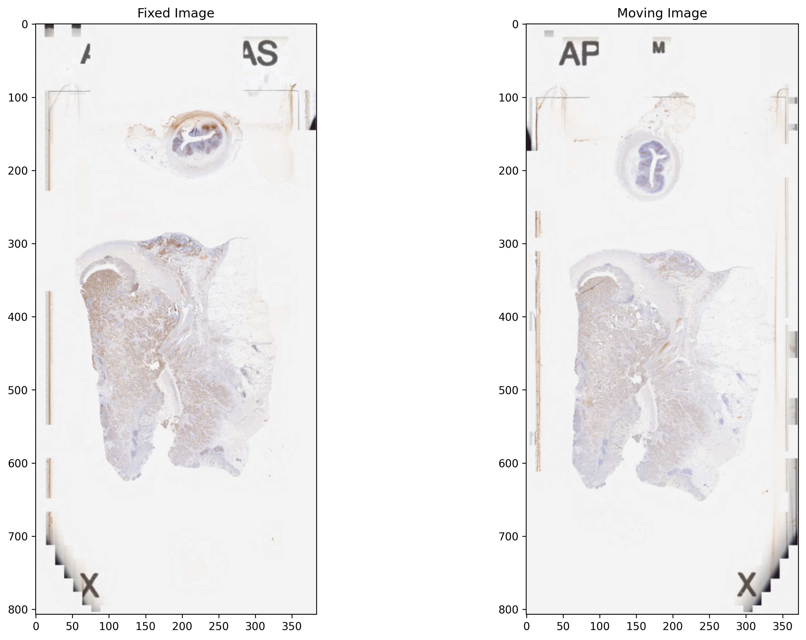
Image Pre-processing

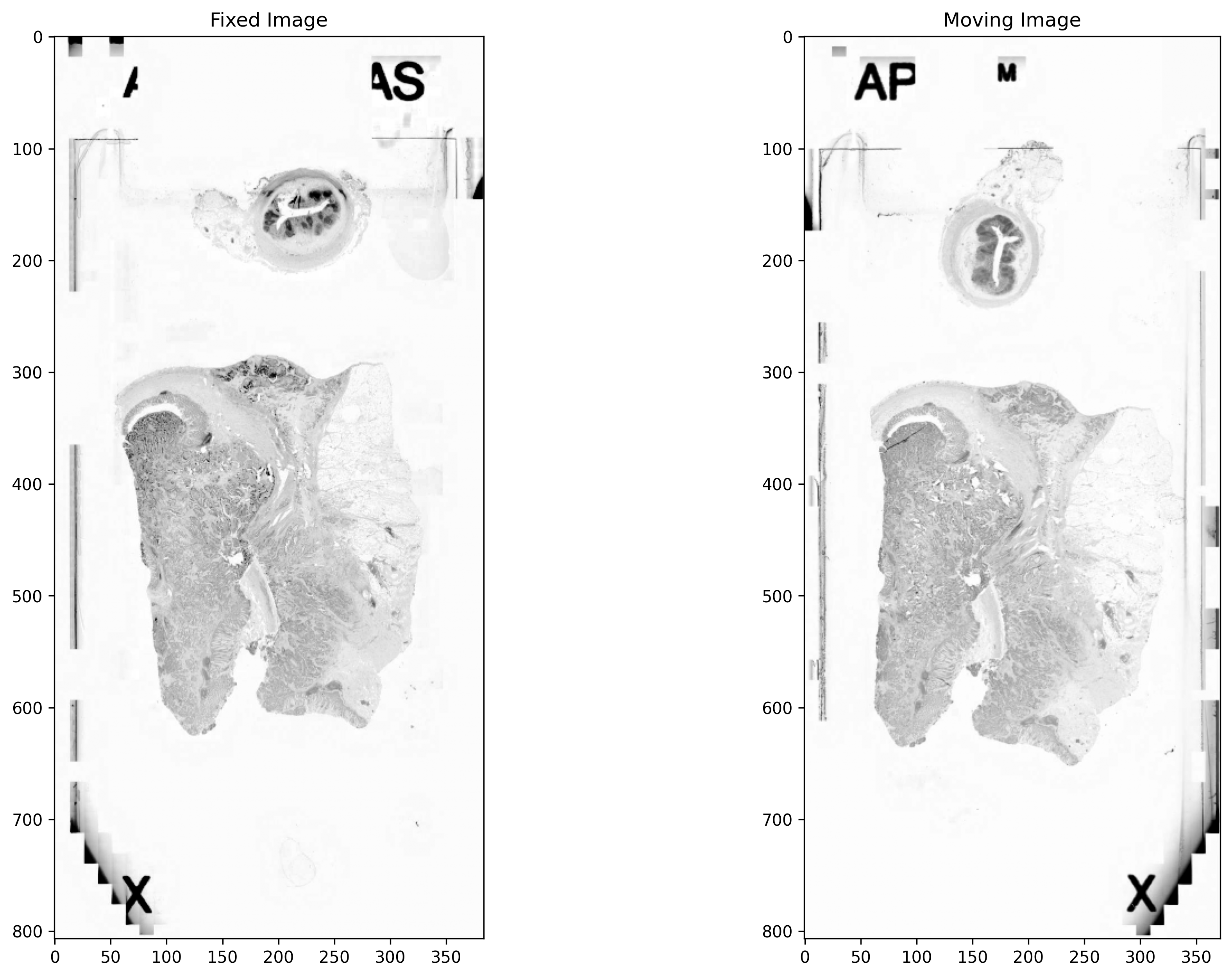
The images are converted to greyscale. The contrast of both the images is improved by linearly rescaling the values. To unify the appearance of an image pair, histogram matching is performed as a normalisation step. In histogram matching, the histogram of an image is modified to be similar to that of another image. An image with high entropy is considered as a reference image and the histogram of an image with low entropy is matched to the reference image.

def preprocess_image(image: np.ndarray) -> np.ndarray:
    """Pre-process image for registration using masks.

    This function converts the RGB image to grayscale image and
    improves the contrast by linearly rescaling the values.

    """
    image = color.rgb2gray(image)
    image = exposure.rescale_intensity(
        image,
        in_range=tuple(np.percentile(image, (0.5, 99.5))),
    )
    image = image * 255
    return image.astype(np.uint8)


# Preprocessing fixed and moving images
fixed_image = preprocess_image(fixed_image_rgb)
moving_image = preprocess_image(moving_image_rgb)
fixed_image, moving_image = match_histograms(fixed_image, moving_image)

# Visualising the results
_, axs = plt.subplots(1, 2, figsize=(15, 10))
axs[0].imshow(fixed_image, cmap="gray")
axs[0].set_title("Fixed Image")
axs[1].imshow(moving_image, cmap="gray")
axs[1].set_title("Moving Image")
plt.show()

temp = np.repeat(np.expand_dims(fixed_image, axis=2), 3, axis=2)
_saved = cv2.imwrite(str(global_save_dir / "fixed.png"), temp)
temp = np.repeat(np.expand_dims(moving_image, axis=2), 3, axis=2)
_saved = cv2.imwrite(str(global_save_dir / "moving.png"), temp)

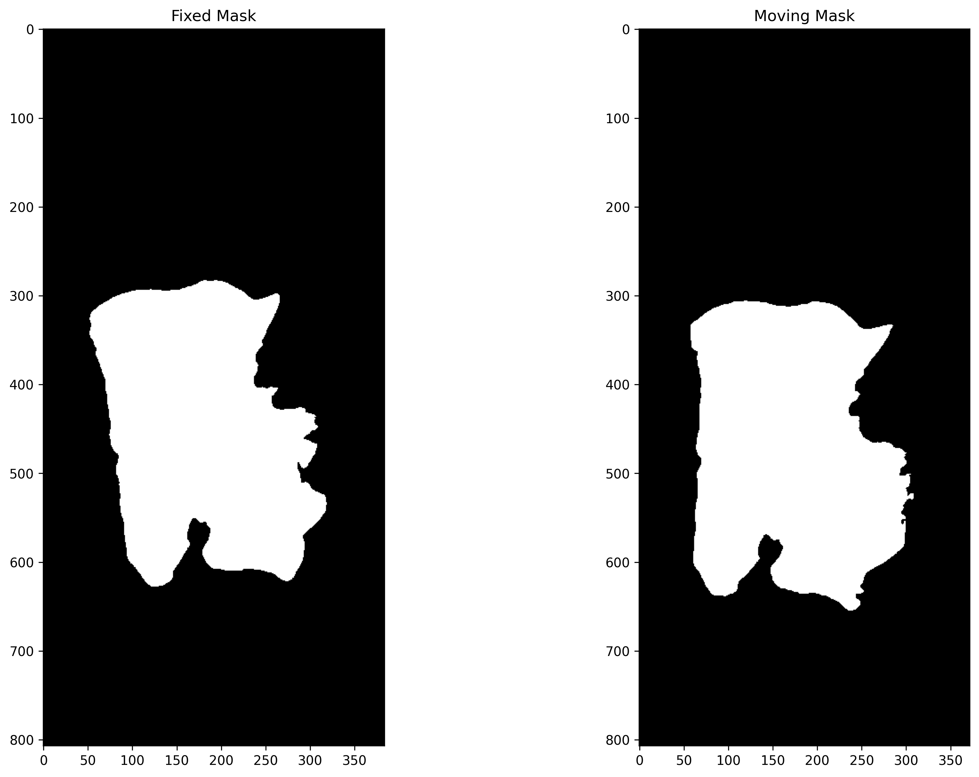
Tissue Segmentation

In this section, image segmentation is performed to generate tissue masks so that registration can be performed using only the active or discriminatory tissue area. In DFBR, these are used to exclude the matching points from the non-tissue and fatty regions while in the non-rigid alignment method, the background region is excluded from images before inputting them to the SimpleITK module.

Here, we use the TIAToolbox semantic segmentor and its built-in model for tissue segmentation. We should mention that when you use a TIAToolbox pretrained model, you don’t need to worry about setting the input/output shape parameters as their optimal values will be loaded by default. For more detailed information on semantic segmentor, readers are referred to a semantic segmentation example notebook.

save_dir = global_save_dir / "tissue_mask"
if save_dir.exists():
    shutil.rmtree(save_dir, ignore_errors=False, onerror=None)

segmentor = SemanticSegmentor(
    pretrained_model="unet_tissue_mask_tsef",
    num_loader_workers=4,
    batch_size=4,
)

output = segmentor.predict(
    [
        global_save_dir / "fixed.png",
        global_save_dir / "moving.png",
    ],
    save_dir=save_dir,
    mode="tile",
    resolution=1.0,
    units="baseline",
    patch_input_shape=[1024, 1024],
    patch_output_shape=[512, 512],
    stride_shape=[512, 512],
    on_gpu=ON_GPU,
    crash_on_exception=True,
)

Post-processing and Visualization of Masks

In the output, the prediction method returns a list of the paths to its inputs and to the processed outputs saved on the disk. This can be used to load the results for processing and visualisation. In this section, a simple processing of the raw prediction is performed to generate the tissue mask.

def post_processing_mask(mask: np.ndarray) -> np.ndarray:
    """Post-process WSI masks."""
    mask = ndimage.binary_fill_holes(mask, structure=np.ones((3, 3))).astype(int)

    # num of unique objects for segmentation is 2.
    num_unique_labels = 2
    # remove all the objects while keep the biggest object only
    label_img = measure.label(mask)
    if len(np.unique(label_img)) > num_unique_labels:
        regions = measure.regionprops(label_img)
        mask = mask.astype(bool)
        all_area = [i.area for i in regions]
        second_max = max([i for i in all_area if i != max(all_area)])
        mask = morphology.remove_small_objects(mask, min_size=second_max + 1)
    return mask.astype(np.uint8)


fixed_mask = np.load(output[0][1] + ".raw.0.npy")
moving_mask = np.load(output[1][1] + ".raw.0.npy")

# num of unique objects for segmentation is 2.
num_unique_labels = 2

# Simple processing of the raw prediction to generate semantic segmentation task
fixed_mask = np.argmax(fixed_mask, axis=-1) == num_unique_labels
moving_mask = np.argmax(moving_mask, axis=-1) == num_unique_labels

fixed_mask = post_processing_mask(fixed_mask)
moving_mask = post_processing_mask(moving_mask)

_, axs = plt.subplots(1, 2, figsize=(15, 10))
axs[0].imshow(fixed_mask, cmap="gray")
axs[0].set_title("Fixed Mask")
axs[1].imshow(moving_mask, cmap="gray")
axs[1].set_title("Moving Mask")
plt.show()

Registration using DFBR

In this section, we apply the DFBR method for aligning the moving image with respect to the fixed image. The pre-trained VGG-16 model is used as a feature extractor which accepts input images with 3 channels. Therefore, greyscale images were stacked as the colour channel. The output of “df.register” is the affine transform which is capable of representing translations, rotations, shearing and scaling.

dfbr_fixed_image = np.repeat(np.expand_dims(fixed_image, axis=2), 3, axis=2)
dfbr_moving_image = np.repeat(np.expand_dims(moving_image, axis=2), 3, axis=2)

dfbr = DFBRegister()
dfbr_transform = dfbr.register(
    dfbr_fixed_image,
    dfbr_moving_image,
    fixed_mask,
    moving_mask,
)

# Visualization
original_moving = cv2.warpAffine(
    moving_image,
    np.eye(2, 3),
    fixed_image.shape[:2][::-1],
)
dfbr_registered_image = cv2.warpAffine(
    moving_image,
    dfbr_transform[0:-1],
    fixed_image.shape[:2][::-1],
)
dfbr_registered_mask = cv2.warpAffine(
    moving_mask,
    dfbr_transform[0:-1],
    fixed_image.shape[:2][::-1],
)

before_overlay = np.dstack((original_moving, fixed_image, original_moving))
dfbr_overlay = np.dstack((dfbr_registered_image, fixed_image, dfbr_registered_image))

_, axs = plt.subplots(1, 2, figsize=(15, 10))
axs[0].imshow(before_overlay, cmap="gray")
axs[0].set_title("Overlay Before Registration")
axs[1].imshow(dfbr_overlay, cmap="gray")
axs[1].set_title("Overlay After DFBR")
plt.show()

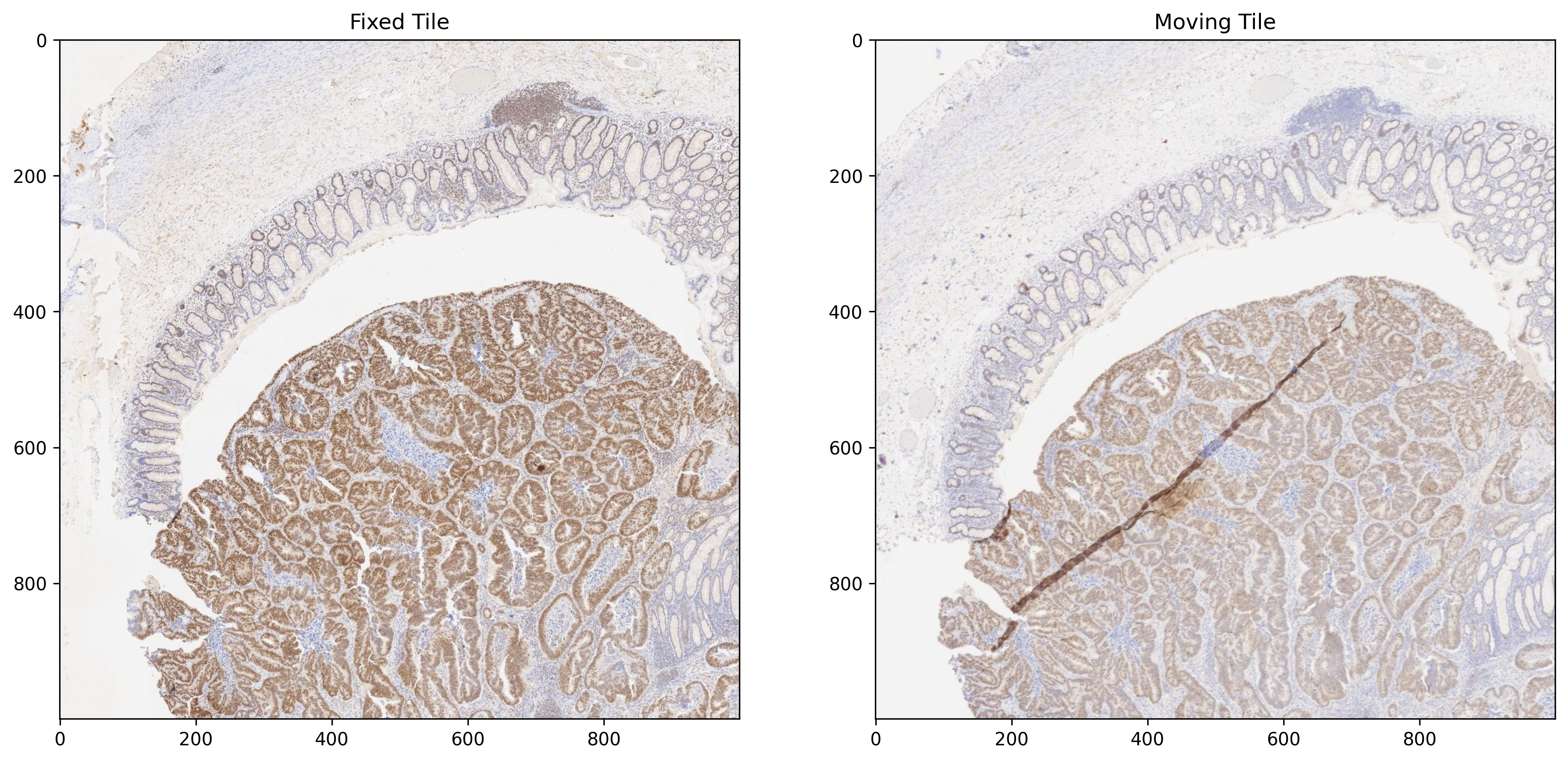
Patch Extraction

In this section, we use the AffineWSITransformer class to extract a region from a fixed image and the corresponding region from a moving image of any size at a specific location of any pyramid level. Using this class, one can extract a transformed tile from a moving image without a need to generate transformed WSI in a pyramidal format. AffineWSITransformer takes two inputs: the WSIReader object for the moving WSI and the transformation matrix at level 0. The transformation is applied for the requested tile only. The read_rect function of the AffineWSITransformer takes the same argument values for extracting region from the moving WSI as the read_rect function of the WSIReader class for extracting region from the fixed WSI.

location = (3500, 20000)  # at base level 0
size = (1000, 1000)  # (width, height)

# Extract region from the fixed whole slide image
fixed_tile = fixed_wsi_reader.read_rect(location, size, resolution=2.5, units="power")

# DFBR transform is computed for level 6
# Hence it should be mapped to level 0 for AffineWSITransformer
dfbr_transform_level = 6
transform_level0 = dfbr_transform * [
    [1, 1, 2**dfbr_transform_level],
    [1, 1, 2**dfbr_transform_level],
    [1, 1, 1],
]

# Extract transformed region from the moving whole slide image
tfm = AffineWSITransformer(moving_wsi_reader, transform_level0)
moving_tile = tfm.read_rect(location, size, resolution=2.5, units="power")

_, axs = plt.subplots(1, 2, figsize=(15, 10))
axs[0].imshow(fixed_tile, cmap="gray")
axs[0].set_title("Fixed Tile")
axs[1].imshow(moving_tile, cmap="gray")
axs[1].set_title("Moving Tile")
plt.show()

Non-rigid registration using B-spline Transform

Histology slides mostly have non-linear deformations that cannot be tackled with a global rigid transformation alone. On the other hand, non-rigid registration methods are capable of finding correspondence by locally transforming a moving image. These methods require two images to be linearly aligned before their application. In this section, we perform non-rigid B-spline registration of linearly aligned fixed and moving tiles using a multi-resolution approach. The moving image here is a registered tile after the application of the DFBR transform, as shown above. For any given image pair, this method is shown to perform better with the inverted intensity values. The B-spline approach involves a number of parameters that the user can experiment with. Changing these parameters would result in varying complexity and registration completion times. For details on the whole list of possible parameters, readers are referred to its documentation. Feel free to play around with the non-rigid alignment parameters and experiment with new images.

fixed_mask = np.ones(shape=fixed_tile.shape, dtype=int)
moving_mask = np.ones(shape=moving_tile.shape, dtype=int)
bspline_transform = estimate_bspline_transform(
    fixed_tile,
    moving_tile,
    fixed_mask,
    moving_mask,
    grid_space=200.0,
    sampling_percent=0.1,
)

Now, we apply the B-Spline transform to the linearly aligned moving tile. To apply the transform, a resampling operation is performed. For comparison purposes, overlaid images of fixed and moving tiles before and after the application of the B-spline transform are presented below.

bspline_registered_image = apply_bspline_transform(
    fixed_tile,
    moving_tile,
    bspline_transform,
)

tile_overlay = np.dstack(
    (moving_tile[:, :, 0], fixed_tile[:, :, 0], moving_tile[:, :, 0]),
)
bspline_overlay = np.dstack(
    (
        bspline_registered_image[:, :, 0],
        fixed_tile[:, :, 0],
        bspline_registered_image[:, :, 0],
    ),
)

_, axs = plt.subplots(1, 2, figsize=(15, 10))
axs[0].imshow(tile_overlay, cmap="gray")
axs[0].set_title("Before B-spline Transform")
axs[1].imshow(bspline_overlay, cmap="gray")
axs[1].set_title("After B-spline Transform")
plt.show()

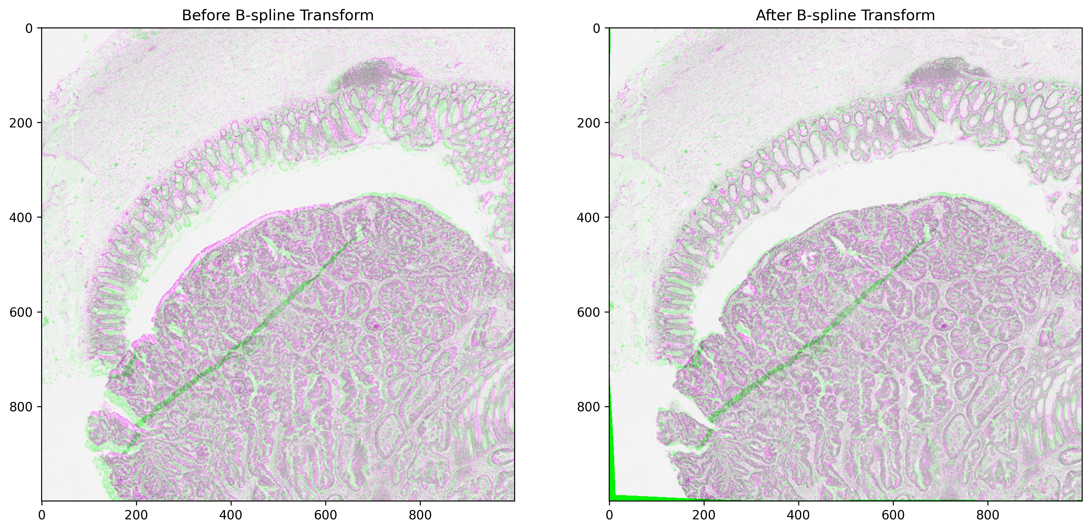
The overlaid image of fixed and moving images on the right side shows a better overlap of histological structures as compared to the overlaid image on the left side. This is because the B-spline approach identifies the local deformations in the tissue and hence further improves the alignment by transforming the moving image locally. The most noticeable improvement can be seen on the bottom left side and at the top of the glandular tissue area.