Read and Visualize a WSI
Click to open in: [GitHub][Colab]
About this demo
This demo reads a whole slide image (WSI) using tiatoolbox. We load a sample WSI, gather some key information, and then extract some image patches. We demo our modules
wsireader details and
slide_info details.
Set Up Plotting
Here we import matplotlib and set some options for plotting results to make the output look nice.
"""Import modules required to run the Jupyter notebook."""

# Clear logger to use tiatoolbox.logger
import logging

if logging.getLogger().hasHandlers():
    logging.getLogger().handlers.clear()

# Pretty print for nice dictionary printing
from pprint import pprint

import matplotlib as mpl
import matplotlib.pyplot as plt

from tiatoolbox import logger
from tiatoolbox.data import small_svs
from tiatoolbox.wsicore.wsireader import WSIReader

mpl.rcParams["figure.dpi"] = 150  # for high resolution figure in notebook
mpl.rcParams["figure.facecolor"] = "white"  # To make sure text is visible in dark mode
plt.rcParams.update({"font.size": 5})
Reading in a WSI
We load a small WSI, specified with the help of the data module. Here we include a function to download a small sample SVS image from our server. This function then returns the path to the downloaded file which is stored in your system’s temporary directory, e.g. /tmp on UNIX-like systems.
file_path = small_svs()
logger.info(file_path)
Our code shields the user from the incompatible formats produced by different models of scanners from different vendors. The function WSIReader.open has as input a particular WSI, with a particular image format, and outputs an object reader, whose base class is WSIReader, and whose derived class depends on the image format (see details). The reader reader provides important information about the WSI. Member functions obtain pixel- or patch-level information, using format-independent code, as we illustrate below.
reader = WSIReader.open(file_path)
print(reader)  # noqa: T201
<tiatoolbox.wsicore.wsireader.OpenSlideWSIReader object at 0x7a54a3f5ddb0>
First, let’s check the basic WSI information, such as magnification, dimension, etc.
(mpp = microns per pixel).
info_dict = reader.info.as_dict()
pprint(info_dict)  # noqa: T203
{'axes': 'YXS',
 'file_path': PosixPath('/tmp/CMU-1-Small-Region.svs'),
 'level_count': 1,
 'level_dimensions': ((2220, 2967),),
 'level_downsamples': [1.0],
 'mpp': (0.499, 0.499),
 'objective_power': 20.0,
 'slide_dimensions': (2220, 2967),
 'vendor': 'aperio'}
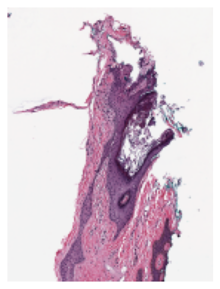
Thumbnail
To see a thumbnail of the WSI, we use the slide_thumbnail method of reader.
We load the thumbnail at $\times1.25$ objective power as follows:
thumbnail = reader.slide_thumbnail(resolution=1.25, units="power")
plt.imshow(thumbnail)
plt.axis("off")
plt.show()
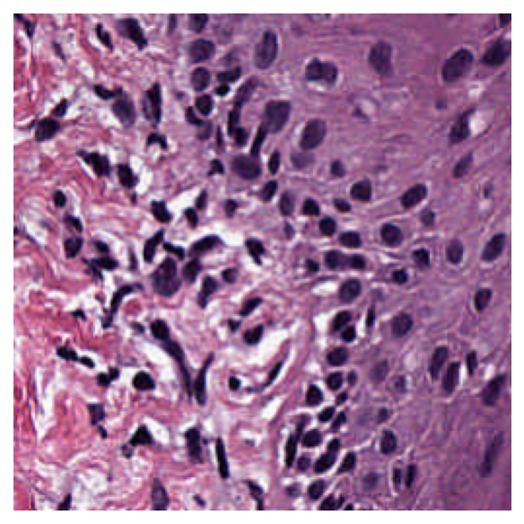
Reading WSI regions
i) Read Rect
We can read a region of the whole slide image at a given location and size using the read_rect method. Location can be stated as (x, y) tuple giving the top left pixel in the baseline (level 0) reference frame, and size as (width, height) tuple giving the desired output image size.
Reads can be performed at different resolutions by supplying a pair of arguments for the resolution and the units of resolution. resolution can be given as integer or float or tuple(float), default = 0. Either a single number or a sequence of two numbers for x and y as tuple are valid. This value is in terms of the corresponding units. For example: resolution=0.5 and units=’’mpp’’ will read the slide at 0.5 microns per-pixel, and resolution=3, units=’’level’’ will read at level at pyramid level / resolution layer 3. Supported units are: microns per pixel (‘’mpp’’), objective power (‘’power’’), pyramid / resolution level (‘’level’’), pixels per baseline pixel (‘’baseline’’), default =’’level’’.
# Location coordinates in (x,y)
location = (1000, 1000)

# Size of the region in (width, height)
size = (256, 256)

# read the region using wsi reader's read rect at 0.5 mpp
img = reader.read_rect(
    location,
    size,
    resolution=0.5,
    units="mpp",
)

plt.imshow(img)
plt.axis("off")
plt.show()
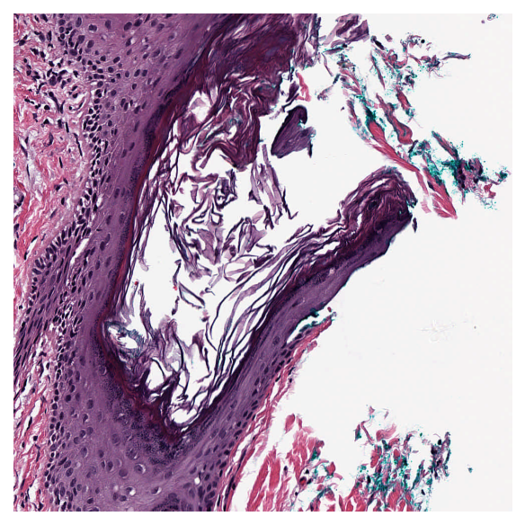
ii) Read bound
Read a region of the whole slide image within given bounds. Bounds is a tuple of (start_x, start_y, end_x, end_y) i.e., (left, top, right, bottom) of the region in baseline reference frame. However, with coord_space=’’resolution’’, the bound is expected to be at the requested resolution system.
Reads can be performed at different resolutions by supplying a pair of arguments for the resolution and the units of resolution. resolution can be given as integer or float or tuple(float), default = 0. Either a single number or a sequence of two numbers for x and y as tuple are valid. This value is in terms of the corresponding units. For example: resolution=0.5 and units=’’mpp’’ will read the slide at 0.5 microns per-pixel, and resolution=3, units=’’level’’ will read at level at pyramid level / resolution layer 3. Supported units are: microns per pixel (‘’mpp’’), objective power (‘’power’’), pyramid / resolution level (‘’level’’), pixels per baseline pixel (‘’baseline’’), default =’’level’’.
coord_space = ‘’baseline’’ by default, this is a flag to indicate if the input bounds is in the baseline coordinate system (‘’baseline’’) or is in the requested resolution system (‘’resolution’’).
# Specify the bounds in terms of rectangle (left, top, right, bottom)
bounds = [1000, 1000, 2000, 2000]

# Read the region using wsi reader's read bounds at level 0
img = reader.read_bounds(bounds, resolution=0, units="level")

plt.imshow(img)
plt.axis("off")
plt.show()
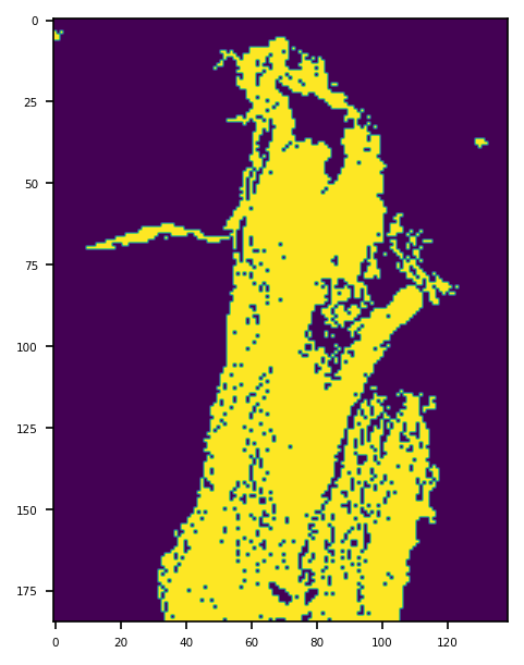
Tissue Masking
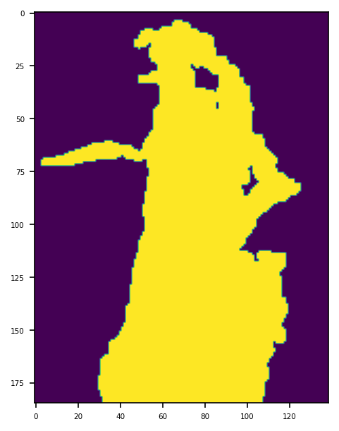
It is often useful to distinguish between tissue and glass (no tissue) in the image. For example, to avoid running computation expensive analysis for regions where is no tissue content. We compute a mask, by which we mean a binary colouring of the pixels to either black=glass or white=tissue. The white area is deliberately made a little larger than tissue area, as this will be appropriate for our task. We provide a function tissue_mask on a WSIReader binarises the thumbnail on the basis of pixel intensity, using the Otsu method. Morphological operations improve the result.
Note that the tissue_mask function returns a VirtualWSIReader object rather than a NumPy array (although this can be accessed via the .image attribute). The returned VirtualWSIReader object also has some metadata copied from the original WSI. This allows the lower resolution mask image to be read as it it were the full size WSI. This is particularly useful as it allows for using the same coordinates to read from the mask as from the original WSI.
mask_reader = reader.tissue_mask(resolution=4, units="mpp")
mask_thumbnail = mask_reader.slide_thumbnail(resolution=1.25, units="power")

plt.imshow(mask_thumbnail)
plt.show()
mask_reader = reader.tissue_mask("morphological", resolution=4, units="mpp")
mask_thumbnail = mask_reader.slide_thumbnail(resolution=1.25, units="power")

plt.imshow(mask_thumbnail)
plt.show()
Here we show reading part of the tissue from reader and also the corresponding part of the mask.
tissue_region = reader.read_rect(
    location=(1500, 1500),
    size=(500, 500),
    resolution=0.5,
    units="mpp",
)
mask_region = mask_reader.read_rect(
    location=(1500, 1500),
    size=(500, 500),
    resolution=0.5,
    units="mpp",
)
_, axs = plt.subplots(1, 2)
axs[0].imshow(tissue_region)
axs[1].imshow(mask_region, vmin=0, vmax=1)
plt.show()
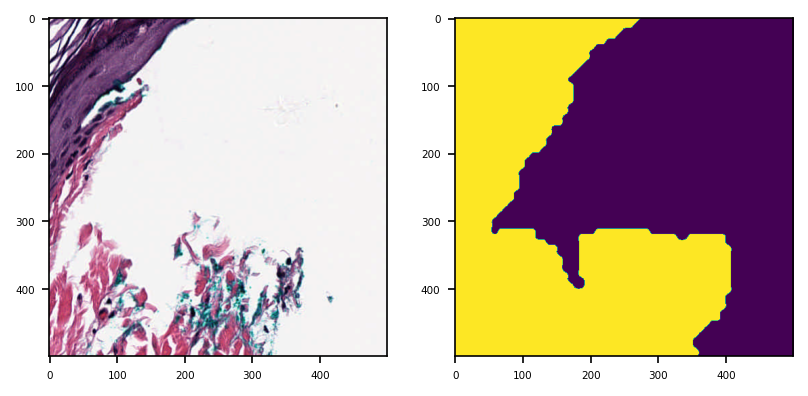
Notice that the above two function calls to the two reader objects have identical arguments. This could also be written more concisely as follows:
# Try modifying the parameters and see how the mask changes
location, size = (1500, 1500), (500, 500)
tissue_region, mask_region = (
    r.read_rect(location, size, 0.5, "mpp") for r in (reader, mask_reader)
)
_, axs = plt.subplots(1, 2)
axs[0].imshow(tissue_region)
axs[1].imshow(mask_region, vmin=0, vmax=1)
plt.show()