Prediction of Molecular Pathways and Key Mutations
Click to open in: [GitHub][Colab]
About this demo
Prediction of molecular pathways and key mutations directly from Haematoxylin and Eosin stained histology images can help bypass additional genetic (e.g., polymerase chain reaction or PCR) or immunohistochemistry (IHC) testing, which can therefore save both money and time.
In this example notebook, we show how you can use pretrained models to reproduce the inference results obtained by Bilal et al.
In this paper, an Iterative Draw and Rank Sampling (IDaRS) approach is proposed, which consists of a two-stage approach:
Patch-level tumour classification
Patch-level WSI classification
In stage 1, we use a pretrained tumour segmentation model to identify potentially diagnositc areas. In stage 2, we make a task-specific prediction for each tumour patch. For stage 2, the model is trained utilising only the slide-level label and hence the model does not require any detailed annotations at the cell or region level. Here, representative tiles from each WSI are iteratively sampled, which gives justification for the name IDaRS.
In TIAToolbox, we include models that are capable of predicting:
Microsatellite instability (MSI)
Hypermutation density
Chromosomal instability
CpG island methylator phenotype (CIMP)-high prediction
BRAF mutation
TP53 mutation
Available models
In line with the above description, in TIAToolbox, we provide the following pretrained models used as part of the original publication.
Tumour segmentation
resnet18-idars-tumour
Task specific prediction
MSI:
resnet34-idars-msiHypermutation density:
resnet34-idars-hmChromosomal instability:
resnet34-idars-cinCpG island methylator phenotype (CIMP)-high prediction:
resnet34-idars-cimpBRAF mutation:
resnet34-idars-brafTP53 mutation:
resnet34-idars-tp53
The provided models are trained on the first fold used in the original paper.
Downloading the required files
We download, over the internet, image files used for the purpose of this notebook. In particular, we download a whole slide image of cancerous colon tissue to highlight how the pipeline works.
In Colab, if you click the files icon (see below) in the vertical toolbar on the left hand side then you can see all the files which the code in this notebook can access. The data will appear here when it is downloaded.

wsi_file_name = save_dir / "sample_wsi.svs"
logger.info("Download has started. Please wait...")

# Downloading sample TCGA whole-slide image
r = requests.get(
    "https://huggingface.co/datasets/TIACentre/TIAToolBox_Remote_Samples/resolve/main/sample_wsis/TCGA-AD-6964-01Z-00-DX1.83AF88B9-C59B-48C6-A739-85ACB8F8ECA9.svs",
    timeout=100,  # 100s
)
with wsi_file_name.open("wb") as f:
    f.write(r.content)

logger.info("Download is complete.")
Tumour segmentation using TIAToolbox pretrained models
In this section, we will display patch-level tumour segmentation results using a pretrained model used in the original paper by Bilal et al. In particular, this model is a ResNet model with 18 layers (resnet18). A prediction is made for each input patch, which denotes the probability of being tumour.
More information on the model and the dataset used for training can be found here.
In line with the patch prediction model provided in TIAToolbox, the tumour segmentation model can be applied to input patches, large images tiles or whole-slide images. In order to replicate the original pipeline, we choose to process a sample whole-slide image. It can be seen that we can perform inference on a WSI with minimal effort. First we create the PatchPredictor object, which denotes the pretrained model that we will use, along with other arguments, such as the batch size and number of workers. Then, we call the predict method to process the slide and return the results. More information on using the PatchPredictor functionality can be seen in the dedicated patch prediction notebook.
save_dir = Path("./tmp/")
wsi_file_name = save_dir / "sample_wsi.svs"
wsi_file_list = [
    wsi_file_name,
]  # the list of WSIs to process- in this example we just use a single WSI.
tumour_predictor = PatchPredictor(
    model="resnet18-idars-tumour",
    batch_size=64,
    num_workers=WORKERS,
)
tumour_output = tumour_predictor.run(
    images=wsi_file_list,
    mode="wsi",
    return_probabilities=True,
    device=device,
    patch_mode=False,
    overwrite=True,
    save_dir=save_dir / "tumour_predictor_output",
)
As can be seen above, with just a few lines of code we are able to perform tumour segmentation on whole-slide images. When running the prediction, as we did above, the default parameters for patch_shape, stride_shape and resolution will be used. Here, patch_shape, and resolution are in line with what was used for training the model, whereas stride_shape is set to be equal to the patch_shape (no overlap). In particular, the input patch size is 512x512 and the processing resolution is 0.5 microns per pixel (~20x objective magnification).
If you want to change the default parameters, you will need to define this using IOPatchPredictorConfig. For example, you may want to run with 50% overlap between neighbouring patches. Therefore, you would define:
wsi_ioconfig = IOPatchPredictorConfig(
    input_resolutions=[{'units': 'mpp', 'resolution': 0.5}],
    patch_input_shape=[512, 512],
    stride_shape=[256, 256],
)
Then, you would add this in the run method as follows:
tumour_output = tumour_predictor.run(
    images=[wsi_file_name],
    patch_mode=False,
    return_probabilities=True,
    device="cuda",
    ioconfig=wsi_ioconfig)
The above result provides the output in a format which is useful for downstream analysis, however, to visualize the results we need the output in a different format.
Visualizing the Results
To visualize the results we can save the output in AnnotationStore or QuPath format. We run the same code above but with the output_type="AnnotationStore".
tumour_output = tumour_predictor.run(
    images=wsi_file_list,
    mode="wsi",
    return_probabilities=True,
    device=device,
    patch_mode=False,
    overwrite=True,
    save_dir=save_dir / "tumour_predictor_output",
    output_type="AnnotationStore",
    class_dict={0: "non-tumour", 1: "tumour"},
)
To visualize the results, run the following command on your local machine after installing TIAToolbox.
%%bash
tiatoolbox visualize --slides ./tmp/ --overlays ./tmp/tumour_predictor_output/
Example Visualization

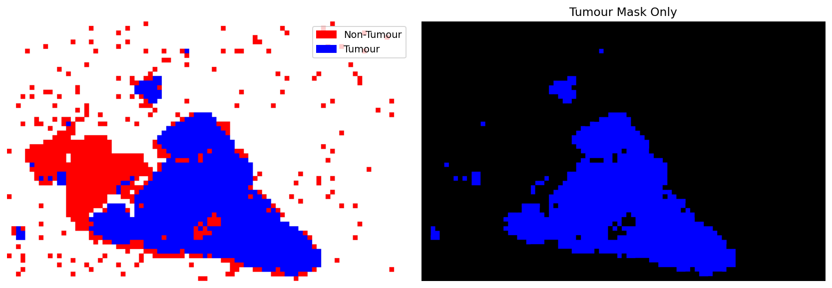
Creating Tumour Mask from Annotations
This can be done directly from AnnotationStore, using AnnotationRenderer and AnnotationStoreReader.
Key Concepts
Color Specification: The mapper dictionary maps annotation types to RGBA colors in the range [0, 1]. These values are internally multiplied by 255 to produce the final pixel values.
"tumour": [0, 0, 1]→ Blue (0, 0, 255)"non-tumour": [1, 0, 0]→ Red (255, 0, 0)Background areas remain white (255, 255, 255)
Interpolation Strategy: When downsampling to create thumbnails, the choice of interpolation method is critical:
interpolation='nearest': Preserves exact categorical colors (no blending)interpolation='area'or'cubic': Creates anti-aliased edges with intermediate colorsFor categorical masks where exact color values matter, use
'nearest'interpolation
Why use read_bounds() instead of slide_thumbnail()?
The slide_thumbnail() method uses default interpolation='optimise' which applies cubic or area interpolation, causing color blending. Using read_bounds() allows explicit control over the interpolation method to preserve distinct colors.
# Step 1: Open the base WSI to get its metadata
wsi_reader = WSIReader.open(wsi_file_name)

# Step 2: Create a renderer with custom color mapping
renderer = AnnotationRenderer(
    score_prop="type",  # Property key to use for coloring annotations
    mapper={
        "tumour": [0, 0, 1, 1],  # Blue: (0, 0, 255, 255) in RGBA
        "non-tumour": [1, 0, 0, 1],  # Red: (255, 0, 0, 255) in RGBA
    },
    max_scale=1000,  # Maximum downsample level for full geometry rendering
    edge_thickness=1,  # Line thickness for annotation boundaries
)

# Step 3: Create an AnnotationStoreReader to render annotations as an overlay
annotation_store_reader = AnnotationStoreReader.open(
    save_dir / "tumour_predictor_output" / "sample_wsi.db",
    info=wsi_reader.info,  # Use WSI metadata for coordinate system
    renderer=renderer,  # Use our custom renderer
)

# Step 4: Generate thumbnail
slide_dimensions = annotation_store_reader.info.slide_dimensions
bounds = (0, 0, *slide_dimensions)  # Read entire slide bounds
thumbnail = annotation_store_reader.read_bounds(
    bounds,
    resolution=1.25,  # Resolution at 1.25x magnification
    units="power",  # Units in objective power
    interpolation="nearest",  # Preserve exact colors
)

# Step 5: Create a binary tumour mask
# Extract only blue pixels (tumour regions), set everything else to black
tumour_mask = np.where(
    np.all(thumbnail == [0, 0, 255], axis=-1, keepdims=True), [0, 0, 255], [0, 0, 0]
).astype(np.uint8)

# Step 6: Visualize both the full annotation thumbnail and the tumour-only mask
fig, axes = plt.subplots(1, 2, figsize=(12, 6))
axes[0].imshow(thumbnail)
axes[0].axis("off")
red_patch = mpatches.Patch(color="red", label="Non-Tumour")
blue_patch = mpatches.Patch(color="blue", label="Tumour")

# 2. Pass these patches to the legend function
axes[0].legend(handles=[red_patch, blue_patch])

axes[1].imshow(tumour_mask)
axes[1].set_title("Tumour Mask Only")
axes[1].axis("off")
plt.tight_layout()
plt.show()


# Step 7: Save the tumour mask for later use
save_path = save_dir / "tumour_mask.png"
imwrite(save_path, tumour_mask)
logger.info("Tumour mask saved to %s", save_path)
|2026-02-27|08:03:44.019| [WARNING] Read: Scale > 1.This means that the desired resolution is higher than the WSI baseline (maximum encoded resolution). Interpolation of read regions may occur.
|2026-02-27|08:03:44.667| [INFO] Tumour mask saved to tmp/tumour_mask.png
WSI prediction using TIAToolbox pretrained models
Next, we show how one can use a second CNN that takes as input the results obtained from part 1 and gives a prediction for each tumour patch in the input WSI. In the original paper, 4 fold cross validation was used. In the toolbox, we choose to provide models trained on the first fold of the data, which enables us to cross check the results and ensure that they are in line with the original work. All models in the second step of the pipeline are ResNet34.
To speed up this step, we choose to retrain the models without stain normalization (as oppoed to the original IDaRS) and instead with colour jitter. We report the difference in results at the end of this notebook.
Near the beginning of the notebook, we mention which prediction tasks we consider. Next, we will run inference for all of these prediction tasks and visualise the output.
# Run inference for each of the 6 WSI prediction tasks
prediction_tasks = ["msi", "braf", "cimp", "cin", "hm", "tp53"]

# iterate over each of the prediction tasks and add the results to a dictionary
wsi_output_dict = {}
for task in tqdm(prediction_tasks, leave=False, desc="Running WSI prediction tasks"):
    wsi_predictor = PatchPredictor(
        model=f"resnet34-idars-{task}",
        batch_size=64,
        num_workers=WORKERS,
    )

    # Obtained tumour mask from stage 1 to only process patches from those regions.
    wsi_output_dict[task] = wsi_predictor.run(
        images=wsi_file_list,
        masks=[save_dir / "tumour_mask.png"],
        patch_mode=False,
        return_probabilities=True,
        device=device,
        overwrite=True,
        save_dir=save_dir / f"{task}_predictor_output",
        output_type="AnnotationStore",
        class_dict={0: f"non-{task}", 1: task},
    )
Visualizing Probability Maps for Multiple Prediction Tasks
With predictions for all six molecular pathways stored as AnnotationStores, we can now create probability heatmap overlays to visualize model confidence across the WSI.
Understanding Probability Map Visualization
What are probability maps? Each patch in the WSI has an associated prediction probability (0-1) stored in the annotation properties. By rendering these with a color gradient, we create a visual heatmap showing where the model is most confident about each molecular marker.
Key visualization parameters:
mapper='jet': Uses the classic rainbow colormap where blue=low probability, red=high probabilityscore_prop='prob_{task}': Specifies which probability value to visualize for coloringwhereclause: Filters to show only patches above a confidence threshold (e.g., prob > 0.1)blur_radius: Applies Gaussian blur to smooth the heatmapalpha=0.5: Sets overlay transparency to blend predictions with the underlying tissue imagebase_wsi: Renders probability maps on top of the actual WSI
This approach provides interpretability by showing which tissue regions contribute most to the overall slide-level prediction.
# Initialize containers and task list
prediction_tasks = ["msi", "braf", "cimp", "cin", "hm", "tp53"]

# Open the base WSI for tissue context
wsi_reader = WSIReader.open(wsi_file_name)

fig, axes = plt.subplots(2, 3, figsize=(14, 7))
axes = axes.flatten()

# Loop through each prediction task and create probability heatmaps
for i, task in enumerate(
    tqdm(prediction_tasks, leave=False, desc="Generating Probability Heatmaps")
):
    # Path to the annotation store containing patch-level predictions
    store_path = save_dir / f"{task}_predictor_output" / "sample_wsi.db"

    # Configure the renderer for probability-based coloring
    renderer = AnnotationRenderer(
        score_prop=f"prob_{task}",  # Use the probability value for this specific task
        mapper="jet",  # Jet colormap
        max_scale=1000,
        edge_thickness=1,
        where=f"props['prob_{task}'] > 0.1",  # Only show patches with >0.1 probability
        blur_radius=5,  # Apply 5-pixel Gaussian blur for smooth heatmap appearance
    )

    # Create reader that overlays the probability heatmap on the base WSI
    annotation_store_reader = AnnotationStoreReader.open(
        store_path,
        base_wsi=wsi_reader,  # Render on WSI
        renderer=renderer,  # Use our own renderer
        alpha=0.5,  # 50% transparency
    )

    # Generate and display the thumbnail with probability overlay
    thumbnail = annotation_store_reader.slide_thumbnail(resolution=1.25, units="power")
    axes[i].imshow(thumbnail)
    axes[i].set_title(f"{task.upper()}")
    axes[i].axis("off")

fig.suptitle("Probability Map Overlay for Each Task")
plt.tight_layout()
plt.show()
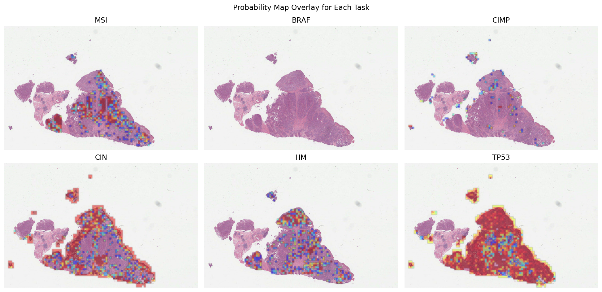
These probability maps can be used to increase the interpretability of results and help identify regions contributing to the overall prediction. To get a smoother output, you can increase the blur_radius by modifying AnnotationRenderer.
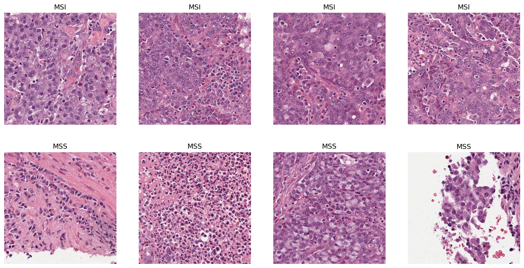
Let’s visualise some patches that have either a high probability or a low probability of being MSI positive. For this, we randomly sample 4 patches with probability of being MSI > 0.95 and 4 patches with probability of being MSI < 0.05.
msi_annotation_store_path = store_path = (
    save_dir / "msi_predictor_output" / "sample_wsi.db"
)
msi_annotation_store = SQLiteStore.open(msi_annotation_store_path)

# subset where MSI probability is greater than 0.95
threshold = 0.95
msi_subset_pos_bbs = msi_annotation_store.bquery(
    where=f"props['prob_msi'] > {threshold}"
)

# subset where MSI probability is less than than 0.05
threshold = 0.05
msi_subset_neg_bbs = msi_annotation_store.bquery(
    where=f"props['prob_msi'] < {threshold}"
)

# randomly sample 4 positive and 4 negative
msi_sample_pos_keys = random.sample(list(msi_subset_pos_bbs.keys()), k=4)
msi_sample_neg_keys = random.sample(list(msi_subset_neg_bbs.keys()), k=4)
Now that we have obtained our random sample, let’s plot the patches! First, we use TIAToolbox’s WSIReader to read the original WSI and extract patches at defined locations. For detailed information on this, see the relevant example notebook!
# read the WSI
wsi_reader = WSIReader.open(input_img=wsi_file_name)

# visualise the overlays in a single plot

fig, axes = plt.subplots(2, 4, figsize=(16, 8))
axes = axes.flatten()

for i, key in enumerate(msi_sample_pos_keys + msi_sample_neg_keys):
    if i < 4:  # noqa: PLR2004
        axes[i].set_title("MSI")
        coords = msi_subset_pos_bbs[
            key
        ]  # get the coordinates of the bounding box for the annotation
    else:
        axes[i].set_title("MSS")
        coords = msi_subset_neg_bbs[
            key
        ]  # get the coordinates of the bounding box for the annotation

    coords = [int(c) for c in coords]  # convert coordinates to integers

    patch = wsi_reader.read_bounds(coords, resolution=0, units="level")
    axes[i].imshow(patch)
    axes[i].axis("off")
plt.show()
The probability maps are not directly needed to obtain the WSI-level score. Below, we will demonstrate how one can obtain the WSI score utilising the output from the PatchPredictor in step 2. For the purpose of this example, we will show how to use mean and max aggregation to obtain a slide-level prediction score.
First, let’s examine the format of the AnnotationStore output by PatchPredictor. We look only at the MSI output as an example, but the output from each task is similar.
annotation = next(
    iter(msi_annotation_store.values())
)  # get the first annotation from the store
logger.info("Annotation geometry: %s", annotation.geometry)
logger.info("Annotation properties: %s", annotation.properties)
|2026-02-27|08:07:47.494| [INFO] Annotation geometry: POLYGON ((39111.11111111111 5333.333333333334, 39111.11111111111 6222.222222222223, 40000 6222.222222222223, 40000 5333.333333333334, 39111.11111111111 5333.333333333334))
|2026-02-27|08:07:47.495| [INFO] Annotation properties: {'prob_non-msi': 0.9800451397895813, 'prob_msi': 0.019954852759838104, 'type': 'non-msi'}
As we can see, the probabilities are stored in Annotation properties. Now, let’s compute, for each task, the average and maximum over all probabilities of tumour tiles being positive.
slide_score_mean = {}
slide_score_max = {}
# iterate over the tasks
for task in prediction_tasks:
    annotation_store = SQLiteStore.open(
        save_dir / f"{task}_predictor_output" / "sample_wsi.db"
    )
    probabilities_query_result = annotation_store.pquery(
        select=f"props['prob_{task}']", unique=False
    )
    slide_score_mean[task] = np.mean(list(probabilities_query_result.values()))
    slide_score_max[task] = np.max(list(probabilities_query_result.values()))
    annotation_store.close()


# print the scores
print("MEAN AGGREGATION")  # noqa: T201
for task, value in slide_score_mean.items():
    print(task, ":", value)  # noqa: T201

print("-" * 30)  # noqa: T201

print("MAX AGGREGATION")  # noqa: T201
for task, value in slide_score_max.items():
    print(task, ":", value)  # noqa: T201
|2026-02-27|08:07:50.930| [WARNING] Query is not using an index. Consider adding an index to improve performance.
|2026-02-27|08:07:51.112| [WARNING] Query is not using an index. Consider adding an index to improve performance.
|2026-02-27|08:07:51.342| [WARNING] Query is not using an index. Consider adding an index to improve performance.
|2026-02-27|08:07:51.585| [WARNING] Query is not using an index. Consider adding an index to improve performance.
|2026-02-27|08:07:51.775| [WARNING] Query is not using an index. Consider adding an index to improve performance.
|2026-02-27|08:07:52.009| [WARNING] Query is not using an index. Consider adding an index to improve performance.
MEAN AGGREGATION
msi : 0.19994407708842657
braf : 0.0012032982876137278
cimp : 0.04632381419772748
cin : 0.49370449357863927
hm : 0.2078893496707449
tp53 : 0.8029315133717888
------------------------------
MAX AGGREGATION
msi : 0.9999943971633911
braf : 0.0461079403758049
cimp : 0.9974960684776306
cin : 0.9994841814041138
hm : 0.9999963045120239
tp53 : 0.9997156262397766
As can be seen, it is straight forward to go from the WSI output to the WSI-level prediction score. In a similar way, different aggregation methods can be used, such as top k probabilities. To highlight how easy it is to obtain the slide level score using TIAToolbox, we provide below the code required to go from input to output.
# TUMOUR DETECTION
tumour_predictor = PatchPredictor(pretrained_model='resnet18-idars-tumour', batch_size=64)

tumour_output = tumour_predictor.predict(
    imgs=[wsi_file_name],
    mode='wsi',
    return_probabilities=True,
    device="cuda")

tumour_mask = tumour_predictor.merge_predictions(
    wsi_file_name,
    tumour_output[0],
    resolution=overview_resolution,
    units=overview_unit)

tumour_mask = tumour_mask == 2 # binarise the output
imwrite(save_dir + 'tumour_mask.png',
    tumour_mask.astype('uint8') * 255)

# WSI PREDICTION
msi_predictor = PatchPredictor(pretrained_model='resnet34-idars-msi', batch_size=64)

msi_output = msi_predictor.predict(
    imgs=[wsi_file_name],
    masks=[save_dir + 'tumour_mask.png'],
    mode='wsi',
    return_probabilities=True,
    device="cuda")

# SLIDE-LEVEL SCORE
msi_probabilities = np.array(msi_output[0]['probabilities'])[...,1] # only consider MSI class
average_msi_probability = np.mean(msi_probabilities) # get the average over all tumour tiles
We encourage you to play around with the models provided by TIAToolbox for prediction of molecular pathways and key mutations. To make a different WSI level prediction, all you need to do is use a different task-specific pretrained weights in the second PatchPredictor.
Below, we report the results obtained with our retrained model compared to the original results. For the purpose of this, we only consider mean aggregation for each task. All results show the area under the receiver operating characteristic curve (AUROC).
| Task | Original | TIAToolbox | | —- | ——– | ———- | | MSI | 0.83 | 0.87 | | TP53 | 0.76 | 0.75 | | BRAF | 0.81 | 0.75 | | CIMP | 0.85 | 0.75 | | CIN | 0.85 | 0.81 | | HM | 0.86 | 0.79 |