Multi-Task Segmentation Models
Click to open in: [GitHub][Colab]
About this demo
In image processing it may be desirable to perform multiple tasks simultaneously with the same model. This may not only have the advantage of decreasing processing time (in comparison to doing the tasks sequentially or separately), but it may also provide complementary information to improve the accuracy of each task. Thus, some multi-task models may actually provide better results than separate models performing the tasks independently. For example, within histology, certain nucleus types may be more prominent in specific tissue regions - e.g. epithelial cells within the epithelium vs. inflammatory cells within the connective tissue. Thus, a model that learns to semantically segment tissue regions at the same time as segmenting/classifying nuclear instances may provide superior results.
In this notebook, we demonstrate how to use HoVer-Net+, a subclass of HoVer-Net, for the semantic segmentation of intra-epithelial layers, whilst simultaneously segmenting/classifying nuclear instances (epithelial, inflammatory etc.). This model has been trained on a private cohort of oral epithelial dysplasia cases (not publicly available). For more information on these individual tasks (e.g. semantic segmentation and nuclear instance segmentation) please see their respective example notebooks. We will first show how this pretrained model, incorporated in TIAToolbox, can be used for multi-task inference on large image patches, before explaining how to use your pretrained model in the TIAToolbox model inference pipeline to do prediction on a set of WSIs.
Setting up the environment
TIAToolbox and dependencies installation
You can skip the following cell if 1) you are not using the Colab plaform or 2) you are using Colab and this is not your first run of the notebook in the current runtime session. If you nevertheless run the cell, you may get an error message, but no harm will be done. On Colab the cell installs tiatoolbox, and other prerequisite software. Harmless error messages should be ignored. Outside Colab , the notebook expects tiatoolbox to already be installed. (See the instructions in README.)
%%bash
apt-get -y install libopenjp2-7-dev libopenjp2-tools libpixman-1-dev | tail -n 1
pip install uv
uv pip install git+https://github.com/TissueImageAnalytics/tiatoolbox.git@develop | tail -n 1
echo "Installation is done."
Downloading the required files
We download, over the internet, image files used for the purpose of this notebook. In particular, we download a histology tile and a whole slide image of cancerous breast tissue samples to show how semantic segmentation models work. Pretrained weights of a Pytorch model and a small WSI are downloaded to illustrate how to incorporate your own models in the existing TIAToolbox segmentation tool.
In Colab, if you click the files icon (see below) in the vertical toolbar on the left hand side then you can see a list of files that have been downloaded and are thus directly accessible from this notebook.

# These file name are used for
img_file_name = global_save_dir / "sample_tile.png"
wsi_file_name = global_save_dir / "sample_wsi.svs"

logger.info("Download has started. Please wait...")

# Downloading sample image tile
download_data(
    "https://huggingface.co/datasets/TIACentre/TIAToolBox_Remote_Samples/resolve/main/sample_imgs/tcga_hnscc.png",
    img_file_name,
)

# Downloading sample whole-slide image
download_data(
    "https://huggingface.co/datasets/TIACentre/TIAToolBox_Remote_Samples/resolve/main/testdata/models/samples/wsi2_4k_4k.svs",
    wsi_file_name,
)

logger.info("Download is complete.")
|2026-02-25|09:21:23.922| [INFO] Download has started. Please wait...
|2026-02-25|09:21:24.573| [INFO] Download is complete.
Multi-Task Segmentation using TIAToolbox pretrained models
In this section, we investigate the use of multi-task models that have already been trained on specific tasks and incorporated in the TIAToolbox. We will particularly focus on HoVer-Net+. In the future we plan to incorporate more models. HoVer-Net+ has an encoder-decoder framework, consisting of multiple decoder branches that allows it to perform multiple tasks simultaneouly. It is therefore assumed that the representation of the input image learned by the encoder, is useful for both donwstream tasks. This model performs two tasks:
It segments out nuclear instances from the given input, whilst assigning them to one of two classes: epithelial nuclei or other nuclei (connective/immune cell etc.).
The model semantically segments tissue regions, classifying each indiviudal pixel of a image tile or WSI, as one of five tissue types:
(Superficial) keratin layer
Epithelial layer
Basal epithelial layer
Other (connective tissue etc.)
Background
Note, the first three tissue classes can be considered as the three layers of the epithelium.
More information on the model and the dataset used for training can be found here (Shephard et al., “Simultaneous Nuclear Instance and Layer Segmentation in Oral Epithelial Dysplasia”).
Inference on tiles
Similarly to the semantic segmentation functionality of the TIAToolbox, the multi-task segmentation module works on both image tiles and structured WSIs. First, we need to create an instance of the MultiTaskSegmentor class which controls the whole process of multi-task segmentation and then use it to do prediction on the input image(s):
# Tile prediction
multi_segmentor = MultiTaskSegmentor(
    model="hovernetplus-oed",
    num_workers=0,
    batch_size=4,
)

tile_output = multi_segmentor.run(
    [img_file_name],
    save_dir=global_save_dir / "sample_tile_results",
    # TIAToolbox v2.0 and above use patch_mode=False to run models on Tiles and WSIs
    patch_mode=False,
    device=device,
    auto_get_mask=False,
    # The image has no metadata, so we need to specify
    # at what mpp (microns per pixel) the image was saved.
    wsireader_kwargs={"mpp": 0.50},
    return_predictions=(True, True),  # Return binary map predictions for both tasks
    overwrite=True,  # Overwrite the output directory if it already exists
)
There we go! With only two lines of code, thousands of images can be processed automatically.
There are many parameters associated with MultiTaskSegmentor. Please see the MultiTaskSegmentor notebook and documentation for more information on these parameters. Here we explain only the ones mentioned above:
model: specifies the name of the pretrained model included in the TIAToolbox (case sensitive). We are expanding our library of models pretrained on various segmentation tasks. You can find a complete list of available pretrained models here. In this example, we use the"hovernetplus-oed"pretrained model, which is the HoVer-Net+ model trained on a private cohort of oral epithelial dysplasia cases.num_workers: as the name suggests, this parameter controls the number of CPU cores (workers) that are responsible for the “loading of network input” process, which consists of patch extraction, preprocessing, and post-processing.batch_size: controls the batch size, or the number of input instances to the network in each iteration. If you use a GPU, be careful not to set thebatch_sizelarger than the GPU memory limit would allow.
After the multi_segmentor has been instantiated as a semantic segmentation engine with our desired pretrained model, one can call the run method to do run the full model pipeline on a list of input images (or WSIs). The run function automatically processes all the images on the input list and saves the results on the disk. The process usually comprises patch extraction (because the whole tile or WSI won’t fit into limited GPU memory), preprocessing, model inference, post-processing and prediction assembly. Here are some important parameters that should be set to use the run method properly:
images: List of inputs to be processed. Note that items in the list should be paths to the inputs stored on the disk.save_dir: Path to the main folder in which prediction results for each input will be stored separately.patch_mode: Whether to treat input as patches (True) or WSIs (False). Default isTrue. The mode of inference is set to'False'for processing plain histology images or structured whole slides images, respectively.device: specify appropriate device e.g., “cuda”, “cuda:0”, “mps”, “cpu” etc.
In the output, the run method returns a dictionary or a list of the paths to the processed outputs saved on the disk. This can be used for loading the results for processing and visualisation.
Now that the processing has finished, let’s use the paths in tile_output to load and examine the output. The output is saved in a zarr file with a list of tasks and output for each task saved under its relevant key.
tile_output = zarr.open(tile_output[img_file_name], mode="r")
# As Hover-Net+ performs two tasks,
# nuclear segmentation and cell type classification, and
# layer segmentation and classification,
# the output will contain two keys,
# "nuclei_segmentation" and "layer_segmentation",
# which correspond to the outputs of the two tasks.
logger.info(f"Output keys: {list(tile_output.keys())}")
|2026-02-24|13:13:31.661| [INFO] Output keys: ['layer_segmentation', 'nuclei_segmentation']
Layer Segmentation
Hover-Net+ performs two tasks. Layer segmentation and Nuclei segmentation. Let’s review the output of layer segmentation first.
layer_map = tile_output["layer_segmentation"]["predictions"][:]
# load input image tile for visualization
tile = imread(img_file_name)

# Create color dictionaries for visualization
semantic_color_dict = {
    0: ("Background", (0, 0, 0)),
    1: ("Other", (255, 165, 0)),
    2: ("Basal", (255, 0, 0)),
    3: ("Epithelial", (0, 255, 0)),
    4: ("Keratin", (0, 0, 255)),
}
# Create the semantic segmentation image (in colour)
semantic_map = np.zeros((layer_map.shape[0], layer_map.shape[1], 3)).astype("uint8")
for idx, (_label, color) in semantic_color_dict.items():
    semantic_map[layer_map == idx] = color

fig2 = plt.figure()
ax1 = plt.subplot(1, 2, 1), plt.imshow(tile), plt.axis("off"), plt.title("Input Image")
ax2 = (
    plt.subplot(1, 2, 2),
    plt.imshow(semantic_map),
    plt.axis("off"),
    plt.title("Layer Segmentation"),
)
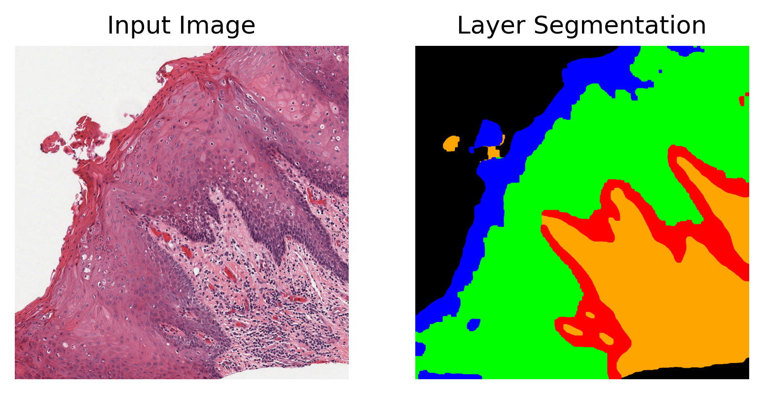
In the layer segmentation prediction map, blue represents the keratin layer, green the epithelial layer, red the basal epithelial layer, orange is other tissue, and finally black is background.
Nuclei Segmentation
The second task is Nuclei Segmentation. Let’s review the output for nuclei segmentation.
nuclei_instances = tile_output["nuclei_segmentation"]

# Log number of detected nuclei.
logger.info(
    "Number of detected nuclei: %d.",
    len(tile_output["nuclei_segmentation"]["contours"]),
)

# Convert the output to the legacy per-instance dict expected by
# overlay_prediction_contours().
inst_dict = {}
for inst_id, (box, centroid, contour, prob, type_id) in enumerate(
    zip(
        nuclei_instances["box"],
        nuclei_instances["centroid"],
        nuclei_instances["contours"],
        nuclei_instances["prob"],
        nuclei_instances["type"],
        strict=False,
    ),
    start=1,
):
    inst_dict[inst_id] = {
        "box": box,
        "centroid": centroid,
        "contour": contour,
        "prob": float(prob) if prob is not None else None,
        "type": int(type_id) if type_id is not None else None,
    }

# Create color dictionaries for visualization
inst_color_dict = {
    0: ("Background", (0, 0, 0)),
    1: ("Other", (255, 165, 0)),
    2: ("Epithelium", (255, 0, 0)),
}

# Create the overlay image
overlaid_predictions_inst = overlay_prediction_contours(
    canvas=tile,
    inst_dict=inst_dict,
    draw_dot=False,
    type_colours=inst_color_dict,
    line_thickness=2,
)

# showing processed results alongside the original images
_ = plt.figure()
ax1 = plt.subplot(1, 2, 1), plt.imshow(tile), plt.axis("off"), plt.title("Tile")
ax3 = (
    plt.subplot(1, 2, 2),
    plt.imshow(overlaid_predictions_inst),
    plt.axis("off"),
    plt.title("Instance segm."),
)
del (
    multi_segmentor,
    tile_output,
    layer_map,
    tile,
    semantic_map,
    overlaid_predictions_inst,
)
gc.collect()  # free up memory
|2026-02-24|13:13:37.404| [INFO] Number of detected nuclei: 3364.
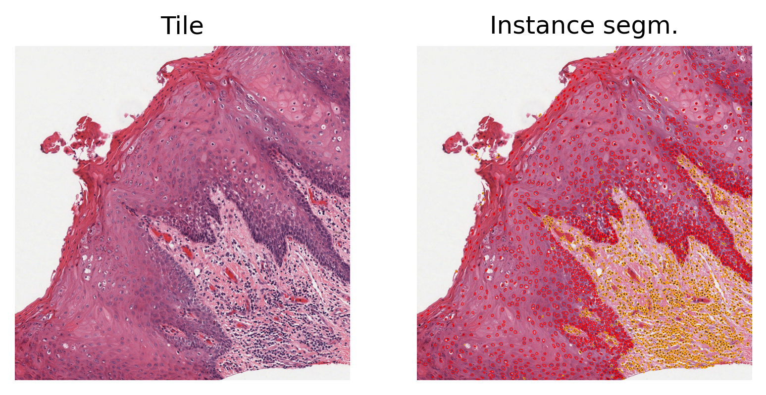
Above, we display the raw image tile, along with the layer segmentation and nuclear instance segmentation predictions. In the instance prediction map, the contours of the nuclear instances are drawn. Red contours represent epithelial nuclei, whilst orange contours represent other nuclei.
Inference on WSIs
The next step is to use TIAToolbox’s embedded model for region segmentation in a whole slide image. The process is quite similar to what we have done for tiles. Here we introduce some important parameters that should be considered when configuring the segmentor for WSI inference. For this example we infer HoVer-Net+ on a small breast tissue WSI.
multi_segmentor = MultiTaskSegmentor(
    model="hovernetplus-oed",
    num_workers=0,
    batch_size=4,
)

# WSI prediction
wsi_output = multi_segmentor.run(
    images=[wsi_file_name],
    masks=None,
    save_dir=global_save_dir / "sample_wsi_results/",
    # TIAToolbox v2.0 and above use patch_mode=False to run models on Tiles and WSIs
    patch_mode=False,
    device=device,
    auto_get_mask=False,
    overwrite=True,  # Overwrite the output directory if it already exists
    return_predictions=(True, True),  # Return binary map predictions for both tasks
)

wsi_output = zarr.open(wsi_output[wsi_file_name], mode="r")
logger.info(f"Output keys: {list(wsi_output.keys())}")
Note the only differences made here are:
Adding
auto_get_mask=Falseto theMultiTaskSegmentor. IfTrueand if nomasksinput is provided to therunfunction, the toolbox automatically extracts tissue masks from WSIs.Setting
patch_mode=Falsein therunfunction indicates that we are predicting region segmentations for inputs in the form of WSIs.masks=Nonein therunfunction: themasksargument is a list of paths to the desired image masks. Patches fromimagesare only processed if they are within a masked area of their correspondingmasks. If not provided (masks=None), then either a tissue mask is automatically generated for whole-slide images or the entire image is processed as a collection of image tiles.
The above cell might take a while to process, especially if you have set device="cpu". The processing time depends on the size of the input WSI and the selected resolution. Here, we have not specified any values and we use the assumed input resolution (20x) of HoVer-Net+.
# [WSI overview extraction]
# Reading the WSI to extract it's overview
wsi = WSIReader.open(wsi_file_name)
logger.info(
    "WSI original dimensions: (%d, %d)",
    wsi.info.slide_dimensions[0],
    wsi.info.slide_dimensions[1],
)

# Reading the whole slide in the highest resolution as a plane image
wsi_overview = wsi.slide_thumbnail(resolution=0.5, units="mpp")
logger.info(
    "WSI overview dimensions: (%d, %d, %d)",
    wsi_overview.shape[0],
    wsi_overview.shape[1],
    wsi_overview.shape[2],
)

layer_map = wsi_output["layer_segmentation"]["predictions"][:]
nuclei_instances = wsi_output["nuclei_segmentation"]

# Convert the output to the legacy per-instance dict expected by
# overlay_prediction_contours().
inst_dict = {}
for inst_id, (box, centroid, contour, prob, type_id) in enumerate(
    zip(
        nuclei_instances["box"],
        nuclei_instances["centroid"],
        nuclei_instances["contours"],
        nuclei_instances["prob"],
        nuclei_instances["type"],
        strict=False,
    ),
    start=1,
):
    inst_dict[inst_id] = {
        "box": box,
        "centroid": centroid,
        "contour": contour,
        "prob": float(prob) if prob is not None else None,
        "type": int(type_id) if type_id is not None else None,
    }

# Create the instance segmentation overlay map
# using the `overlay_prediction_contours` helper function
overlaid_inst_pred = overlay_prediction_contours(
    canvas=wsi_overview,
    inst_dict=inst_dict,
    draw_dot=False,
    type_colours=inst_color_dict,
    line_thickness=4,
)

overlaid_layer_pred = overlay_prediction_mask(
    wsi_overview,
    layer_map,
    alpha=0.5,
    label_info=semantic_color_dict,
    return_ax=False,
)

fig = (
    plt.figure(),
    plt.imshow(wsi_overview),
    plt.axis("off"),
    plt.title("Large Visual Field"),
)
fig = (
    plt.figure(),
    plt.imshow(overlaid_inst_pred),
    plt.axis("off"),
    plt.title("Instance Segmentation Overlaid"),
)
# Create semantic segmentation overlay map
# using the `overlay_patch_prediction` helper function
fig = plt.figure()
plt.imshow(overlaid_layer_pred)
plt.axis("off")
plt.title("Semantic Segmentation Overlaid")

del (
    multi_segmentor,
    wsi_output,
    wsi_overview,
    overlaid_layer_pred,
    overlaid_inst_pred,
    nuclei_instances,
    layer_map,
)
gc.collect()  # free up memory
|2026-02-24|13:13:59.875| [INFO] WSI original dimensions: (4000, 4000)
|2026-02-24|13:14:01.060| [INFO] WSI overview dimensions: (2016, 2016, 3)
Text(0.5, 1.0, 'Semantic Segmentation Overlaid')
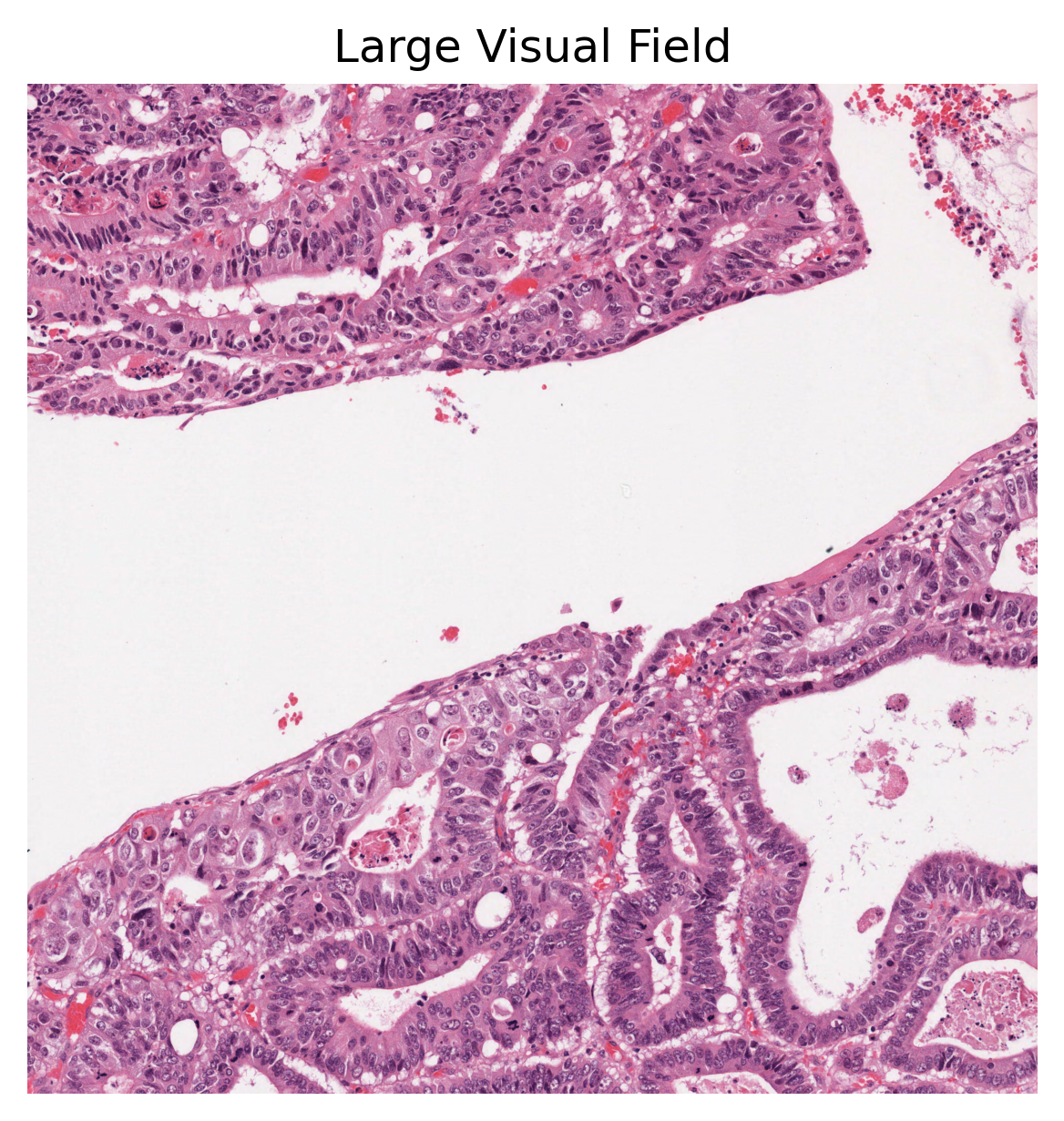
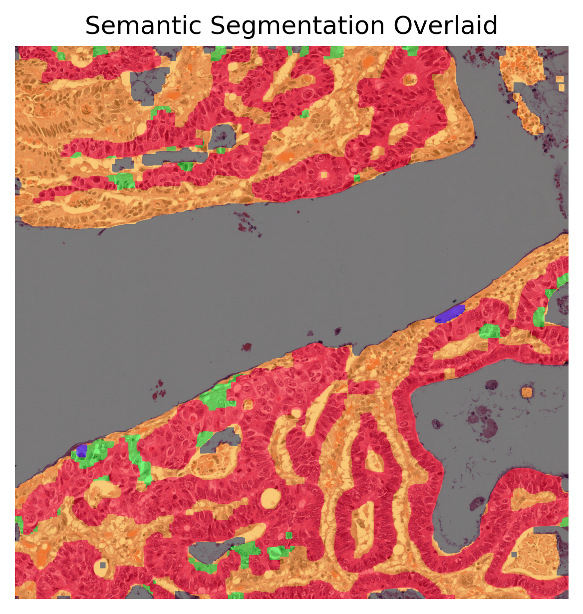
As you can see above, our method first creates the semantic and instance segmentation maps (and corresponding dictionaries). Then, in order to visualise the segmentation prediction on the tissue image, we read the processed WSI and extract its overview. Please note that HoVer-Net+ assumes a base resolution of 0.50 mpp, whilst the baseline resolution of the input WSI was 0.252 mpp. Thus, the output of HoVer-Net+ has shape 2016 x 2016, compared to the input 4000 x 4000. The overview image is therefore also extracted at this resolution. We did not edit this into the processing of the tile as the tile processing assumes the correct input resolution at baseline.
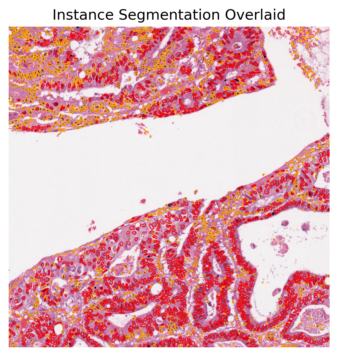
We used the overlay_prediction_mask helper function of the TIAToolbox to overlay the predicted semantic segmentation map on the overview image and depict it with a colour legend. We also used the overlay_prediction_contours helper function of the TIAToolbox to overlay the predicted instance segmentation map on the overview image.
In the instance prediction map, the contours of the nuclear instances are drawn. Red contours represent epithelial nuclei, whilst orange contours represent other nuclei. In the semantic segmentation prediction map, blue represents the keratin layer, green the epithelial layer, red the basal epithelial layer, orange is other tissue, and finally black is background. Please note that the semantic segmentation output seen above is relatively spurious in areas as a result of the model being trained on head and neck tissue only (specifically within oral epithelial dysplasia). However, the WSI inferred on is from breast tissue and thus the model does not generalise well to this task. We have chosen to include this WSI, despite the results not being perfect, for demonstration purposes.
In summary, it is very easy to use pretrained models in the TIAToolbox to do predefined tasks. In fact, you don’t even need to set any parameters related to a model’s input/output when you decide to work with one of TIAToolbox’s pretrained models (they will be set automatically, based on their optimal values).
Feel free to play around with the parameters, models, and experiment with new images (just remember to run the first cell of this notebook again, so that the created folders for the current examples are removed. Alternatively, change the save_dir parameters in new calls of predict function). Currently, we are extending our collection of pre-trained models. To keep track of them, make sure to follow our releases. You can also check here. Furthermore, if you want to use your own pretrained model for semantic segmentation (or any other pixel-wise prediction models) in the TIAToolbox framework, you can follow the instructions in our example notebook on advanced model techniques to gain some insights and guidance.
We welcome any trained model in computational pathology (in any task) for addition to TIAToolbox. If you have such a model (in Pytorch) and want to contribute, please contact us or simply create a PR on our Github page.
How to visualize in TIAViz
TIAToolbox provides a flexible visualization tool for viewing slides and overlaying associated model outputs or annotations. It is a browser-based UI built using TIAToolbox and Bokeh. Below we show how to use this tool for our prediction example.
Note: To visualize the images and output on TIAViz, we recommend running the following code locally on your machine instead of Google Colab.
Note: We have updated the output_type="annotationstore", which is the required output format to visualize the output of models in TIAViz.
multi_segmentor = MultiTaskSegmentor(
    model="hovernetplus-oed",
    num_workers=0,
    batch_size=4,
)

# WSI prediction
wsi_output = multi_segmentor.run(
    images=[wsi_file_name],
    masks=None,
    save_dir=global_save_dir / "sample_wsi_results/",
    # TIAToolbox v2.0 and above use patch_mode=False to run models on Tiles and WSIs
    patch_mode=False,
    device=device,
    auto_get_mask=False,
    overwrite=True,  # Overwrite the output directory if it already exists
    return_predictions=(False, False),  # Binary map predictions not required.
    return_probabilities=False,  # Probability maps not required.
    output_type="AnnotationStore",  # Set to QuPath for direct use in QuPath
)

del multi_segmentor, wsi_output
gc.collect()  # free up memory
Above, we run the MultiTaskSegmentor on WSI file wsi_file_name similar to previous runs, but this time we specify a different value for the parameter output_type (output_type = "AnnotationStore"). In this case, the prediction results will be saved as .db files which are directly compatible with TIAViz.
To start the TIAViz, simply use the command below, either in a terminal or by running the cell, and view localhost:5006 in your web browser.
%%bash
tiatoolbox visualize --slides ./tmp/ --overlays ./tmp/sample_wsi_results/
An example view you will have in your web browser is shown below. Make sure to click on Add Overlay button to select the corresponding overlay (sample_wsi.db) for your WSI (sample_wsi.svs). Try using different colors and changing options.
More details on visualization Interface usage can be found on [Visualization Interface Usage Documentation].
Example TIAViz Visualization
